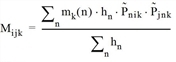
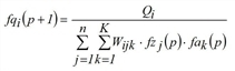
In gravity models, trip distribution or destination choice is made according to the bilinear approach (for example Kirchhoff 1970), using various evaluation or utility functions Wij.

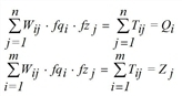
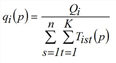
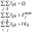
Hereby Tij is the number of trips from i to j, Wij is the cost function for the trip from i to j, Qi is the production of zone i and Zj is the attraction of zone j. The factors fqi, fzj are calculated so that productions and attractions are kept as marginal sums.
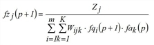
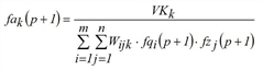
The EVA model generalizes this approach of a simultaneous trip distribution and mode choice to a trilinear model.

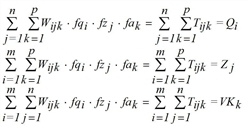
Here, index k is the mode (means of transport) and Wijk assesses the costs for the trip from i to j by modes k. For each demand stratum c there is a separate equation system to be solved independently. For more clarity index c has been dropped for all variables in the problem formulations above.
For the trilinear case, besides origin and destination traffic, the total number VKk of trips with mode k is required. There are two possibilities.
- If EVA trip distribution and mode choice for the analysis case is performed, which means without having run a pre-calculation for the same study area, specify the modal split as input data.
- If, however, a forecast case is calculated, the modal split of the analysis case can be re-used. You thus assume that the modal split may change on single relations, but modal split of the whole model (including all relations), however, remains unchanged.
The problem formulation is applicable in case of hard constraints. For weak, elastic or open constraints equations will be replaced by inequations in the side conditions or a side condition will be dropped completely. This will be dealt with when describing the problem solutions.
The models can be justified by the probability theory using Bayes‘ axiom or the information gain minimization. Both ways lead to the same result.
Minimizing the gain of information has the target that the deviations from a priori assessments of trip relations which would lead to the actually desired trips road users have to experience are as minor as possible, but which have become necessary due to the constraints of the system.
The demand matrix T can be interpreted as the solution to the convex optimization task
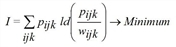
with 
taking account of the constraints. The solution is the trilinear equation system previously determined.
The parameter I represents the information gained through the replacement of distribution wijk (solely determined by the weighting matrix) by distribution pijk (additionally derived from marginal totals).
Weighting probabilities (impedance functions)
In general, the total trips costs include various factors (e.g. journey time, egress/access time, monetary costs, number of passenger transfers etc.). In the EVA model, these are called assessment types. In the EVA model the different assessments of each assessment type are transformed separately by a utility function and then multiplied.
If caijk is the assessment of type a of a trip from i to j by mode k, then the following applies:
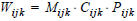
where

Here Mijk stands for the availability of mode k on OD pair (i,j) and Cijk for the capacity utilization of mode k on (i,j). a‘, a‘‘ and a‘‘‘ are the predefined assessment types: journey time, competing walk time and external weighting matrix. A is the number of user-defined assessment types.
Mijk and Cijk are defined independently from the demand stratum as follows:
|
OD type |
Definition of Mijk and Cijk |
|
Type 1 |
Mijk = mk(i) for all j, i.e. value of zone attribute mk set for source zone i Cijk = ck(j) for all i, i.e. value of zone attribute ck set for destination zone j |
|
Type 2 |
Mijk = mk(j) for all i, i.e. value of zone attribute mk set for destination zone j Cijk = ck(i) for all j, i.e. value of zone attribute ck set for source zone i |
|
Type 3 |
without accounting for home zone Mijk = 1 for all i,j,k Cijk = ck(i) • ck(j) including accounting for home zone
Cijk = ck(i) • ck(j) whereby hn stands for the home trips of zone n,
|
 represents the product matrix from the top, but the predefined assessment type External weighting matrix is not included in the product:
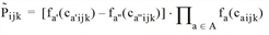
Table 65: Definition of the mode availability and capacity utilization according to the OD type
For demand strata of the origin-destination type 3 (which are calculated accounting for the home zone), the assessment type External weighting matrix is used to produce a specific weighting between zones and modes. This weighting has an immediate impact on the total product, since it is not part of the scaling using home zones, as in the formula for Mijk. In all other cases, this assessment type has the same effect as a user-defined one.
You can use different function types as fa evaluation functions. All distribution functions of the gravity model can be taken, but additionally the EVA1, EVA2, Schiller and Box-Tukey functions (Gravity model calculation) too.
|
|
|
|
|
|
|
|
|
|
|
|
|
|
|
|
|
|
|
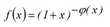
f(x)=exp(c∙α) whereby |
|
|
|
|
|
|
|
|
None |
f(x) = x |
 where
where 


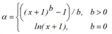
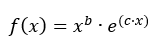

Table 66: Function types for evaluation
In practice particularly the functions EVA1 and EVA2 have proved to be suitable. The EVA1 functions are monotonously falling with f(w) ≤ 1 for w ≥ 0. Some of them have been illustrated in Image 64. Their parameters can be interpreted geometrically.
|
a |
Parameter marking the horizontal asymptote of function φ(w), thus influencing the degree of approximation of the function f(w) to the w asymptote. |
|
b |
Parameter influencing the degree of approximation to the horizontal F(w)=1 in the proximity of low assessment |
|
c |
Parameter influencing the slope of the function f(w) |
|
b/c |
Position of the inflection point WP=F/G of function Φ(w) where the function Φ(w) features the greatest rise or the highest "impedance sensitivity" |
Table 67: Parameters of the evaluation function EVA1
The related elasticity functions are determined by
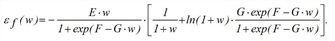
The elasticity function  is defined as the limit of the quotient of the relative variation of the function f and the relative variation of the impedance w.
It is obvious that the elasticity functions first take values near zero for low impedances, then for a limited range in which the “impedance sensitivity“ is at its highest take various values, but all far from zero and for high impedances “approximate“ the limit of -E.
Thus, this curve very much differs from the constant or linear elasticity functions of simple power and exponential functions. Therefore, this type of function allows the adaptation to various basic weighting situations (person groups, trip purposes, means of transport etc.). In the range of low assessment or utility the weighting probability should be almost one, drop further in the clearly noticeable range of assessment and utility which is relevant for the respective type of traffic or purpose before asymptotically approximating zero. For example, the assessment in the proximity of or in smaller towns plays a minor or no role at all for the road users when choosing the destination or the means of transport (here mainly the random model with WP = 1 is applicable).
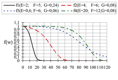

Image 64: EVA1 function dependent on impedance w
The EVA2 function has the following parameters.
|
a, b ... |
Exponents whose product determines the asymptotic behavior for high impedance values. For b > 1 the curve is similar to that of the EVA function (1). |
|
c ... |
Scale parameter for impedance values.
|
 applies.
Table 68: Parameters of the evaluation function EVA2
The Image 65 shows the influence of a and b on the progression of the function. The two other parameters are both kept constant.
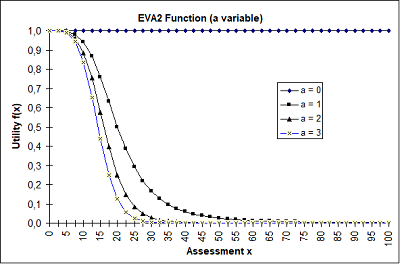

Image 65: EVA2 function dependent on the parameters a and b
The Schiller function is a special case of the EVA2 function, however, with one parameter less. As the first applications in practice have shown, the function can also be adapted sufficiently well enough to observed data. Due to the lower number of parameters the calibration effort is by far lower than for EVA2.
Problem solution 1: The trilinear FURNESS method
The mostly investigated method for solving bilinear problems in technical literature is named after K. P. Furness (Furness 1962, 1965). However, in fact, Bregman had already applied this method in the thirties (Bregman 1967a, 1967b). It can be generalized and transferred directly to the trilinear case.
After you have specified start values for the trilinear FURNESS method

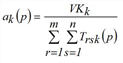
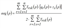
during iteration step p (p=1,2,...), the system calculates approximations for fqi, fzj and fak as follows.
 (i = 1,…,m)
 (j = 1,…,n)
 (k = 1,…,K).
For convergence of the method (towards the solution of the trilinear problem), the condition for unique solvability of the optimization problem is necessary and sufficient, i.e. existence of a matrix Tijk that matches the constraints and for which Tijk = 0 is true for all pairs (i,j) with Wij = 0. This condition is fulfilled when Wij > 0 is true for all (i,j), since then the matrix with elements (the matrix that corresponds to the random model) can be chosen as a feasible solution. For this special case A. W. Evans provided a convergence proof that also allows for a (however rough) estimation of the convergence rate (Evans 1970). The practical experience has shown that the method quickly converges in most application cases.
Problem solution 2: The trilinear Multi method
Another possibility to solve the problem is to set separate fixed point equations for the vectors fqi, fzj and fak and use them to derive rules for determining successive approximations for these vectors (Schnabel 1997). The Multi-Procedure can also be extended to the three dimensional case (Projection). Approximations for the solution of the trilinear problem then can be determined according to the following iteration rule.

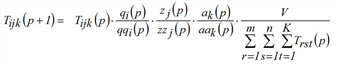
(p = 1, 2,…)
with


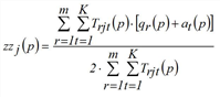
Strictly speaking the method presented solves the problem with hard constraints only. If some constraints are weak or elastic, there will be an optimization problem with inequations as side conditions instead of equations. At the example of weak constraints it is illustrated how the problem and correspondingly its solution alters (according to Schiller 2004). It is assumed that a demand stratum shows weak constraints on the destination side, which means attraction calculated by trip generation constitutes an upper limit. Thus, the trilinear problem changes into

under the constraints
The procedure for multi-problem solving is mostly identical with the constraint equation method, except that zj(p) and zzj(p) are calculated differently.

If some demand strata do not feature hard constraints, not only has the method to be adapted but also balancing has to be made up.
|
Note: Differences in marginal sums can only be balanced after trip generation if all demand strata feature hard constraints. |
In that case first of all the trilinear problem is solved for all demand strata except for the balancing one. This results in the total productions and attractions of the zones covering these demand strata and all modes. According to the formula for calculating productions and attractions (EVA trip generation) the productions and attractions of the balancing demand stratum are modified. Finally Visum runs trip distribution and mode choice for this last demand stratum, too.
The proceeding assumes that differences have to be balanced within the framework of the total volume. This is only true if all modes are exchangeable, which means if they can be used alternatively in a closed trip chain. If at least one mode cannot be exchanged, a second phase begins after the total balancing in which calculations are performed for each non-exchangeable mode separately and for all exchangeable modes jointly. Hereby, the productions and attractions of the respective modes are calculated over the non-balancing demand strata, their differences are compensated by an adaptation of the demand of the balancing demand stratum, and based on that modified demand Trip distribution and Mode choice are calculated for the last time. For non-exchangeable modes this last step corresponds to a simple mode choice.
The implementation of the EVA model for trip distribution and mode choice has been established in two separate operations. EVA Weighting operation uses skim matrices to calculate the weighting matrices Wijk (one weighting matrix each per demand stratum). During EVA trip distribution and Mode choice, the equation systems for determining the demand matrices are set up according to the constraints of the demand strata and solved by applying one of the above-described methods. The result of the operation is one demand matrix per demand stratum and mode. You can also display the balance factors for productions and attractions fqi and fzj, that result from the equation system. The balance factor for mode choice fak is calculated for analysis, but not for forecast scenarios.
The EVA weighting procedure can be applied to all active OD pairs or only to those OD pairs whose origin or destination zone are active. This allows you to perform an analysis based on filtering by several OD pairs with different parameters. This option is not available for combined distribution and mode choice, as for successful balancing, all traffic types need to be accounted for in one step.
