The Gravity model is a mathematical model for trip distribution calculation (Trip distribution and Tour-based model: trip distribution / mode choice combined). It is based on the assumption that the trips made in a planning area are directly proportional to the relevant origin and destination demand in all zones and the functional values of the utility function between the zones (Ortúzar 2001).
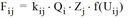
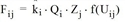
The gravity model calculates a complete matrix of traffic relations Fij, using the OD pairs of marginal totals (origin and destination traffic of the individual zones). A consistent utility matrix of the planning region is required.
The gravity model works with distribution parameters, therefore with values within the utility function, which map the reaction of road users to distance or time relations. These parameters are determined by comparing the demand per OD pair arising from the model, with the counted demand per OD pair (calibration).
The capability of the models to predict future conditions (forecasting) depends on whether they manage to predict the behavior of road users in relation to the network impedances, as well as knowledge of the model input data applicable for the future (for example future travel demand).
|
General form of the distribution formula
|
|
|
Logit |
|
|
Kirchhoff |
|
|
Box-Cox |
|
|
Combined |
|
|
TModel |
|
 where
where


The distribution formula is referred to an attraction or utility function, with the following parameters.
|
Uij |
Value for the utility between zones, for example distance or travel time from zone i to zone j |
|
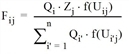
Qi |
Origin zone i |
|
Zj |
Destination zone j |
|
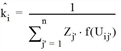
kij |
Scaling factor (attractiveness factor) for OD pair zone i to zone j |
|
n |
Number of zones |
Determining the scaling factor kij and formulating the utility function f(Uij) are essential for various modifications and extensions.
The scaling factor kij must be chosen so that the boundary conditions of the distribution models

and

are (at least approximately) fulfilled.
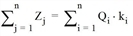
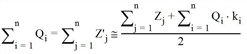
Retaining only the first direction of distribution, we speak of production distribution. Retaining only the second direction of distribution, we speak of attraction distribution. Retaining both directions of distribution at the same time, we speak of doubly-constrained. For coupling in terms of production kij only depends on i, so we write  .
.
For logical reasons, coupling for production requires that there are as many free parameters as there are zones.
This leads to the formulation
with the following secondary conditions for zone i.

From the n secondary conditions, all  can thus be determined by substitution in the distribution function:

This results in
 for Qi ≠ 0
This produces a destination choice model of production distribution.
 for all i, j
The destination choice model of attraction distribution is derived analogously.
 for all i, j with
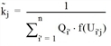
The adjustment of the model to reality (calibration) by variation of the free parameters is very important.
Since the input parameters Qi and Zj have been specified, the only free parameters that remain besides the scaling factors ( and
and  ) are the parameters of the utility function f(Uij).
Since for doubly-constrained calculation both directions of the distribution, [4.1] and [4.2] must be met at the same time, the following must also apply for the scaling factors  and
and  as well as
  =
=  for i = j. In practice, however, this can seldom be achieved, so a true doubly-constrained calculation can only be achieved with much more complex iteration models.
As an iteration model the Matrix Editor uses the so-called Multi procedure according to Lohse (Schnabel 1980) (The multi-procedure according to Lohse (Schnabel 1980)).
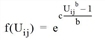
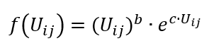
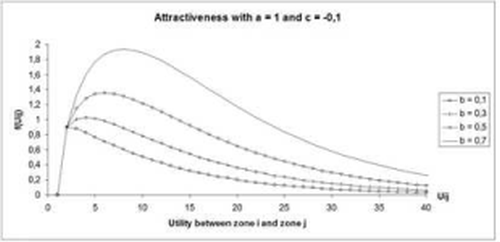
The general form of the utility function f(Uij) is

It is depicted for several b and c parameters in the following two figures.

|
Notes: Choose a suitable specification for the utility functions, which means suitable parameters. Among other things, the specification depends on the trip purpose and the mode used. A trip to work is for example, on average longer than a trip for shopping. This means that the utility function for the trips to work does not depend on utility (distance or travel time) at all, or only to a small extent, depending on the size of the town. Shopping trips on the other hand, are much more dependent on the utility. The use of a trip distribution model can therefore call for a separation of the travel demand based on the trip purpose. This depends essentially on the requirements in terms of accuracy and the demands on the matrix to be calculated. Benchmark figures for the percentage split based on the trip purpose can be obtained for example from the MiD (Mobilität in Deutschland) (BMVBS 2010) or local surveys. |
The following four examples show gravity models that are differently constrained and with and without balancing.
Example 1: Gravity model singly-constrained in terms of production, with and without balancing
The effect of the location factor on the calculation of the trip distribution according to the gravity model depends on the type of “coupling” of the gravity model.
With the distribution method that includes coupling for EITHER attraction or production, the source or destination traffic is adjusted to the marginal totals in the code file. The location factor then only affects the "complementary" destination or origin demand. However,
 or
or 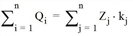
whereby ki or kj are attractiveness factors of the i or j zone.
With the distribution method that includes coupling for attraction AND production, the impact of the attractiveness factor on the origin and destination traffic depends on the function command in the code file. If for example $GQH is given as function command, the origin demand is changed by the location factor that is listed in the same line as the factor within the code file. However,
with ki being the attractiveness factor of the i zone.
- Input file Utility
* Zone numbers
1 2 3 4
* 2.66 1.75 1.99 1.50
* 1 2.08
1.00 0.50 0.33 0.25
* 2 2.33
0.33 0.50 1.00 0.50
* 3 1.41
0.33 0.25 0.33 0.50
* 4 2.08
1.00 0.50 0.33 0.25
* 7.90
*Zone Production Attraction Factor External
1 10.0000 50.0000 0.50000000 0
2 20.0000 10.0000 1.00000000 0
3 30.0000 20.0000 1.00000000 0
4 40.0000 20.0000 1.00000000 1
The parameters are set as follows:
- Combined utility function (exponential)
- Parameter b = 0,5 and c = -1
- Singly-constrained for production without balancing
- Output
* Zone numbers
1 2 3 4
* 36.76 15.91 30.79 16.55
* 1 10.00
3.11 1.45 2.80 2.64
* 2 20.01
6.76 2.81 4.82 5.62
* 3 30.00
9.97 3.76 7.98 8.29
* 4 40.00
16.92 7.89 15.19 0.00
* 100.01
*Zone Production Attraction Factor External
1 10.0000 50.0000 0.50000000 0
2 20.0000 10.0000 1.00000000 0
3 30.0000 20.0000 0.30000000 0
4 40.0000 20.0000 1.00000000 1
The parameters are set as follows:
- Direction of the distribution according to the production distribution with boundary sum balancing enforced by the multi procedure.
- Combined utility function (exponential)
- Parameter b = 0.5 and c = -1
- Scaling according to mean value of both sums
- Max. number of iterations = 10, Quality factor = 3
- Output
* Zone numbers
1 2 3 4
* 32.99 13.19 7.92 26.39
* 1 8.04
2.22 0.94 0.56 4.32
* 2 16.10
4.62 1.74 0.93 8.81
* 3 24.16
6.95 2.38 1.57 13.26
* 4 32.19
19.20 8.13 4.86 0.00
* 80.49
Example 2: Gravity model singly-constrained for production, with balancing
- Input file Utility
* Zone numbers
1 2 3 4 5
* 166.183 107.560 88.972 134.710 155.725
* 1 165.571
0.001 22.700 35.183 50.387 57.300
* 2 107.414
22.700 0.001 15.991 31.017 37.705
* 3 90.008
35.926 16.284 0.001 15.153 22.644
* 4 134.633
50.387 31.017 15.153 0.001 38.075
* 5 155.524
57.169 37.558 22.644 38.152 0.001
* 653,150
*Zone Production Attraction
1 18990.0 18990.0
2 4960.0 4960.0
3 7110.0 7110.0
4 16080.0 16080.0
5 2300.0 2300.0
Location factor and zone property external are not specified. Default values are used.
The parameters are set as follows:
- Direction of the distribution according to the production distribution with boundary sum balancing enforced by the multi procedure.
- Combined utility function (exponential)
- Parameter b = 0.5 and c = -1
- Scaling according to the production total
- Max. number of iterations = 10, Quality factor = 3
- Output
* Zone numbers
1 2 3 4 5
* 18990.000 4959.951 7109.758 16080.290 2300.000
* 1 18990.000
18990.000 0.000 0.000 0.000 0.000
* 2 4959.999
0.000 4959.897 0.102 0.000 0.000
* 3 7110.000
0.000 0.054 7109.426 0.520 0.000
* 4 16080.000
0.000 0.000 0.230 16079.770 0.000
* 5 2300.000
0.000 0.000 0.000 0.000 2300.000
* 49439.999
Example 3: Gravity model singly-constrained for attraction, without balancing
- Input file impedances
* Zone numbers
1 2 3 4
1.00 0.50 0.33 0.25
0.33 0.50 1.00 0.50
0.33 0.25 0.33 0.50
1.00 0.50 0.33 0.25
*Zone Production Attraction
1 10 50
2 20 10
3 30 20
4 40 20
The parameters are set as follows:
- Singly-constrained for attraction, without balancing
- Combined utility function (exponential)
- Parameter b = 0.5 and c = -1
- kj = 1 for all j
This produces the following function values of utilities f(Uij)
Zone 1 2 3 4
1 0,37 0,43 0,41 0,39
2 0,41 0,43 0,37 0,43
3 0,41 0,39 0,41 0,43
4 0,37 0,43 0,41 0,39
and so 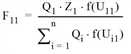

F11 = 4.71
The matrix is produced after the other 15 equations have been calculated.
- Output
* Zone numbers
1 2 3 4
* 50.00 10.00 19.99 19.99
* 1 9.68
4.71 1.03 2.04 1.90
* 2 20.47
10.58 2.06 3.64 4.19
* 3 31.09
15.87 2.80 6.13 6.29
* 4 38.74
18.84 4.11 8.18 7.61
* 99.98
The desired values for destination demand were very well approximated, while the values for origin demand were not reached so well. This circumstance is characteristic for such distribution formulas. Either the origin or the destination sums are reached close enough. If both constraints are to be aligned as closely as possible, it is necessary to use a boundary compensation model. The function doubly-constrained projection (Multi-Procedure) is suitable for this purpose (Projection).
Example 4: Gravity model singly-constrained for attraction, with balancing
Now the trip distribution in Example 3 (Example 3: Gravity model singly-constrained for attraction, without balancing) shall be calculated using a balancing procedure (Multi-procedure).
- Input file impedances
* Zone numbers
1 2 3 4
1.00 0.50 0.33 0.25
0.33 0.50 1.00 0.50
0.33 0.25 0.33 0.50
1.00 0.50 0.33 0.25
* ZoneNo Productions Attractions
1 10 50
2 20 10
3 30 20
4 40 20
The parameters are set as follows:
- Direction of the distribution according to the production distribution with boundary sum balancing enforced by the multi procedure.
- Combined utility function (exponential)
- Parameter b = 0.5 and c = -1
- Scaling according to mean value of both sums
- Max. number of iterations = 10, Quality factor = 3
- Output
* Zone numbers
1 2 3 4
* 50.00 10.01 20.00 20.00
* 1 10.01
4.87 1.06 2.11 1.97
* 2 20.00
10.34 2.01 3.55 4.10
* 3 30.00
15.32 2.70 5.91 6.07
* 4 40.00
19.47 4.24 8.43 7.86
* 100.01
