The functionality is primarily used if origin or destination total values of a zone are to be multiplied by a particular value, or a particular expected value is to be attained, which can be necessary in some circumstances after origin-destination studies. Matrices collected are often just random samples and must be projected to census values.
Matrix values can be projected per row (singly-constrained projection regarding the production), per column (singly-constrained projection regarding the attraction) or by row and column (doubly-constrained projection) (User Manual: Projecting matrix values).
Singly-constrained projection means that each row or column is multiplied by a fixed value. This value can be a procedure parameter or – for zone and main zone matrices – an attribute of the zone or main zone. The complexity of doubly-constrained projection is illustrated in the example below.
Objective: projection of origin and destination demand as follows:
- zone 1 by 10 %
- zone 2 by 20 %
|
Zone |
1 |
2 |
Origin demand |
|
1 |
20 |
30 |
50 |
|
2 |
40 |
50 |
90 |
|
Destination demand |
60 |
80 |
140 |
Line by line multiplication, therefore for purely singly-constrained projection of the demand regarding production originating from zone 1 by 10% and zone 2 by 20%, produces the following matrix.
|
Zone |
1 |
2 |
Origin demand |
|
1 |
22 |
33 |
55 |
|
2 |
48 |
60 |
108 |
|
Destination demand |
70 |
93 |
163 |
While the origin traffic has been increased correctly, the destination traffic has not.
For the doubly-constrained projection, the Matrix editor uses an iterative process, also called a Multi-procedure. During this iterative procedure, a solution to how the target values are best reached is generated stepwise (The multi-procedure according to Lohse (Schnabel 1980)).
The Matrix Editor thus provides the following solution which correctly projects the origin and destination traffic.
|
Zone |
1 |
2 |
Origin demand |
|
1 |
21 |
34 |
55 |
|
2 |
45 |
62 |
107 |
|
Destination demand |
66 |
96 |
162 |
The multi-procedure according to Lohse (Schnabel 1980)
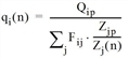
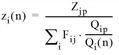
With the multi-procedure new traffic flows are calculated in each iteration step Fij (Schnabel 1980).
The iteration formula applied is as follows
Fij(n+1) = Fij(n) • qi(n) • zj(n) • f(n)
with

|
Qip |
Desired origin traffic zone i |
|
Zjp |
Desired destination traffic zone j |
|
Gp |
Desired total traffic |
|
Fij(n) |
Traffic flow from zone i to zone j in iteration n |
|
Qi(n) |
Origin traffic zone i, iteration n |
|
Zj(n) |
Destination traffic zone j, iteration n |
|
G(n) |
Total traffic, iteration n |
This iterative calculation is done repeatedly until the following conditions are met for all boundary values (origin and destination expected values).
 for all zones i
 for all zones j
The threshold ε suggested by Lohse was used. It states that
 or
or 
QF: quality factor
