In the EVA model and Standard 4-step model, productions and attractions are calculated similarly, namely based on demographic (number of inhabitants) and structural (jobs, size of retail sales floor…) parameters as well as on mobility rates (taken from statistical surveys on traffic behavior). It is performed separately for each demand stratum, which means for each activity pair and its major person groups.
In EVA trip generation productions and attractions normally refer to a closed time interval with regard to traffic (generally the average working day). The following model stages, EVA Weighting and EVA Trip distribution and Mode choice, too, refer to the overall period. The demand matrices available at the end of the model chain only can be combined with an empirically determined or standardized daily time series (Image 62) to get the shares of demand for the individual times of the day. The daily time series depend on the demand stratum.

Image 62: Daily time series for origin-destination groups of HW and WH (SrV 1987 Dresden)
The following table shows the allocation of activities, activity pairs, structural properties and person groups on demand strata. Thereby the abbreviations used stand for the following: H: Home; W: Work; C: Child care facility, S: School; F: Shift; P: Shopping; R: Recreation; O: Others.
|
From/To |
H |
W |
C |
S |
F |
P |
R |
O |
|
H |
|
HW |
HC |
HS |
HF |
HP |
HR |
HO |
|
W |
WH |
|
|
|
|
|
|
WO |
|
C |
CH |
|
|
|
|
|
|
|
|
S |
SH |
|
|
|
|
|
|
|
|
F |
FH |
|
|
|
|
|
|
|
|
P |
PH |
|
|
|
|
|
|
|
|
R |
RH |
|
|
|
|
|
|
|
|
O |
OH |
OW |
|
|
|
|
|
OO |
Table 46: Typical break-down of a demand stratum into 8 activities and 17 demand strata = activity pairs
|
Demand stratum |
Structural property (S) / Person group (P) of source zone i |
|
|
HW |
P |
Employees |
|
HC |
P |
Young children |
|
HS |
P |
Pupils, apprentices, students |
|
HF |
P |
Employees |
|
HP |
P |
Inhabitants |
|
HR |
P |
Inhabitants |
|
HO |
P |
Inhabitants |
|
WO |
S |
Jobs |
|
WH |
S |
Jobs |
|
CH |
S |
Jobs / capacity |
|
SH |
S |
Jobs / capacity |
|
FH |
S |
Jobs |
|
PH |
S |
Jobs / sales floor |
|
RH |
O |
Jobs / capacity |
|
OH |
S |
Other jobs |
|
OW |
S |
Other jobs |
|
OO |
S |
Other jobs |
|
DStr |
Structural property (S) / Person group (P) of destination zone j |
|
|
HW |
S |
Jobs |
|
HC |
S |
Jobs / capacity |
|
HS |
S |
Jobs / capacity |
|
HF |
S |
Jobs |
|
HP |
S |
Jobs / sales floor |
|
HR |
S |
Jobs / capacity |
|
HO |
S |
Other jobs |
|
WO |
S |
Other jobs |
|
WH |
P |
Employees |
|
CH |
P |
Young children |
|
SH |
P |
Pupils, apprentices, students |
|
FH |
P |
Employees |
|
PH |
P |
Inhabitants |
|
RH |
P |
Inhabitants |
|
OH |
P |
Inhabitants |
|
OW |
S |
Jobs |
|
OO |
S |
Other jobs |
Table 47: Examples of relevant structural properties and person groups of the demand strata
Thus, for the demand strata HW and WH only the Employees person group (which could be broken down into further subgroups) is relevant, whereas for the demand strata HO and OH generally all person groups are relevant. The number of persons of all person groups in each zone make up an important part of input attributes for the trip generation of a certain demand stratum. Further structural properties measure the intensity of the activities at the origin or destination. An example of the allocation of certain structural properties to individual demand strata is illustrated in Table 47.
The person groups specified here can be broken down into further subgroups according to other features (car availability, age) and used for trip generation.
For each demand stratum and each relevant person group, mobility rates have to be defined. The mobility rate of a person group is defined as the average number of trips per day and person.

In most cases, the MRpc values are known from national surveys on traffic behavior and are assumed to be constant for all zones of the study area. If the individual zones feature different specific traffic demands, for example distinguishing between urban and rural areas, they can be used, too. Then MRepc specifies the particular demand of the person group or reference person group p in zone e (in a certain demand stratum c).
Analogously production rates − defined as the number of trips per day and structural property − are determined for the major structural properties like number of jobs, sales floor, etc. To do so empirical studies or available historical values can be referred to. Here, too, a differentiation according to zones is possible. The structural potential of the zone results from the value of the structural property and the related production rate.
A certain number of trips of the total production of a zone remains within the study area only, the rest targets destinations outside. The same holds for destination traffic. Since the EVA Model usually serves the calculation of study area-internal traffic (incoming and outgoing traffic as well as through-traffic are often added by other sources), the share of trips of the total origin (or destination) traffic made within the study area can be determined for all origin (or destination) zones.
Example: The origin traffic of the demand stratum of Home-Work (HW) results from the number of persons of the person group of Employees (EP) and the mobility rate MREP,HW. In a zone R on the edge of a study area, however, part of the employees will commute to destination zones outside the study area. It is not available for a later trip distribution and mode choice. In that case, the study area factor UR,EP,HW is below 1, conveying that only that share of trips remains within the study area. For a zone Z in the center, however, all trips of the demand stratum lie within the study area. Therefore the following applies: UZ,EP,HW = 1. Study area factors do not only depend on the zone but also on the demand stratum and the person group. It is more probable that employees with car (E+c) commute over great distances – and therefore to destinations outside the study area than those without car (E-c). If you differentiate these two person groups in the model, then would typically be UR,E-c,HW > UR,E+c,HW. And in analogy hereto would be UR,Child,HC > UR,E+c,HW, because child care facilities are rather found in the proximity of homes than jobs.
As the mobility rate of a person group the production rate of a structural property, too, can have partial impacts in the study area only. So, for example, the structural potential of the demand stratum HW is determined by the number of jobs (structural property J) and the related production rate. On the edge of the study area part of the jobs are taken by employees living outside the study area. Therefore, these jobs are not available as potential destinations of HW trips of the study area. Therefore, in that case, too, the total structural potential is multiplied by a study area factor VR,J,HWA < 1.
You can limit calculation to the active zones. This allows you to e.g. exclude cordon zones from the calculation.
In the trip generation stage (Table 48, Table 49 and Table 50) from the structural data and values mentioned for all demand strata c, the productions Qic and attractions Zjc or the upper limits Qicmax and Zjcmax of these demands are calculated.
The approach depends on the origin-destination type of the activity pair of the demand stratum. It specifies whether the activity pair affects the home activity of the road user as origin or destination. Three types are possible.
- Type 1: origin activity = home activity (own apartment, own work)
- Type 2: destination activity = home activity (own apartment, own work)
- Type 3: origin and destination activity ≠ home activity
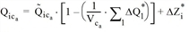
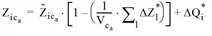
The calculation specifications can be taken from Table 48, Table 49 and Table 50. For the types 1 and 2 calculation starts with the home trips (of number of persons, mobility rate, study area factor) which independently from the travel direction always occur in the origin zone. For type 1 the number of trips corresponds exactly to the production, for type 2 to the attraction of the respective zone. For type 1 the total production (of all zones) is distributed onto the destination zones, in proportion to their potentials (taken from structural properties, production rates and study area factors). Type 2 is treated equally. The total attraction is distributed proportionally to the potentials onto the origin zones. For type 3 total volume is equally calculated on the basis of the total home trips. However, the sizes of the road users’ origin zones are relevant, which do not have to correspond with origin or destination of the trip. Proportionally to the potential the total volume is then distributed onto the origin zones on the one hand and onto the destination zones on the other hand.
The productions and/or attractions so calculated can have various meanings.
- Hard constraints
Traffic demand solely results from the spatial structure and has to be fully exhausted by the trips calculated in the model.
Example: if the number of employed inhabitants and jobs per zone is known, hard constraints will be applicable to the demand stratum Home – Work (HW), since every employed person necessarily has to commute to work and each job has to be destination of commutation.
- Weak constraints
Traffic demand does not only depend on the spatial structure but also on the convenience of the location and the resulting “competitive conditions“. In these cases traffic demands resulting from trip generation are like upper limits. Only trip distribution and mode choice will determine the extent to which the limits will be exhausted by the actual origin and/or destination traffic determined.
The structural potential of the destination zone for the demand stratum Home – Shopping (HP) is usually calculated based on the structural property of sales floor and a production rate for example. It is conceivable that there may be overabundance of sales floor so that the shopping facilities are not used to their full potential. Therefore, the attraction calculated by trip generation from the potential only constitutes an upper limit for real destination traffic. Therefore, the constraint is hard on the destination side, whereas weak on the origin side, because each road user has to shop (somewhere).
- Elastic constraints
Elastic constraints are a generalization of weak constraints. Additionally to upper limits lower limits are equally known, for the demand stratum Home - Shopping (HP), for example, from sales statistics. In this case, the structural potential of the sales floor determines an interval for the attraction of the respective zone.
- Open constraints
The potential of the structure properties merely expresses the attractiveness of the zone as an origin or destination of the demand stratum. However, the production or attraction is not linked to a constraint condition.
The attractiveness of some destinations in recreational traffic can even be measured by means of their attributes if capacity impacts do not play a role. For example, the structural potential of a nearby recreational area can be determined by its forest. During trip distribution this attractiveness is to impact as potential of the destination zone, but no constraints are linked herewith because there is neither a minimum number of persons seeking recreation nor do visitors go to other places, because the "capacity" of the forest is fully exhausted.
The scope of the constraints is defined by selecting the corresponding activity pair attribute Couple DStrata together:
- calculate separately
The constraints are met on the origin and destination side for each demand stratum.
- couple jointly on origin side
The constraints are met on the origin side for all demand strata with this pair of activities.
- couple jointly on destination side
The constraints are met on the destination side for all demand strata with this pair of activities.
- couple jointly on both sides
The constraints are met on the origin and destination side for all demand strata with this pair of activities.
The constraints are loosened by binding them across demand strata. Imagine the following example: There are two groups of people. One of them mainly uses cars, the other mainly uses public transport. Plus there are two origins and two destinations as well as a single activity pair "home - work" of the origin-destination type 1 with strict constraints on the destination side. One of the two destinations is easily accessible by car, the other by public transport.
If destination binding is used without coupling together, both destinations are approached equally by both groups of people, although one would expect the destination choice to be based on reachability via the preferred means of transport.
This is precisely what happens when you couple jointly on the destination side: people of the public transport group will preferably head for the destination that is easily reachable by public transport, while people of the passenger car group will preferably head for the other destination.

Image 63: Result of destination-bound coupling of constraints
Zone "Work A" with good public transport connections was mainly visited by public transport affine persons, while zone "Work B" was mainly visited by car affine persons. Overall, the destination side constraints (100 paths per zone) were met.
|
Note: If you want to validate the data, note that the specified constraints per zone are not fulfilled by the attraction or production of each individual demand stratum when using the coupling, but only apply to the totaled values. |
In Table 48, Table 49 and Table 50 the calculation formulas are listed up separately for the cases for which they differ. Coupling together is not taken into account in the calculation formulas.
|
Step 1 |
Home trips H
|
|
Step 2 |
Production Q, Qmax
|
|
Step 3 |
Total volume V
|
|
Step 4 |
Attraction Z, Zmax
|


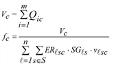
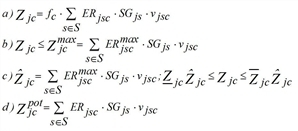
Table 48: Trip generation in EVA model: OD type 1
|
Step 1 |
Home trips H
|
|
Step 2 |
Attraction Z, Zmax
|
|
Step 3 |
Total volume V
|
|
Step 4 |
Production Q, Qmax
|
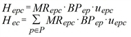


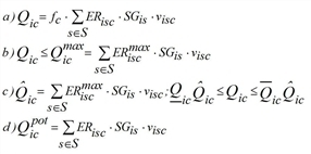
Table 49: Trip generation in EVA model: OD type 2
|
Step 1 |
Home trips H
|
|
Step 2 |
Total volume V
|
|
Step 3 |
Production Q, Qmax
Attraction Z, Zmax
|


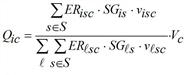
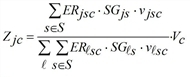
Table 50: Trip generation in EVA model: OD type 3
|
e |
Index of a zone producing trips (origin zone) |
|
i |
Index of a zone being origin of trips |
|
j |
Index of a zone being destination of trips |
|
s |
Index of a structural property |
|
p |
Index of a person group |
|
c |
Index of a demand stratum |
|
m |
Number of zones in study area |
|
MRepc |
Mobility rate of person group p per time interval |
|
ERisc |
Production rate of structural property s per time interval |
|
BPep |
Number of persons per person group p |
|
SG |
Structural property |
|
uepc |
Factor of trips realized study area-internally |
|
visc |
Structural property factor effective for study area-internal traffic |
|
Hepc |
Home trips (expected value) of person group p |
|
Hec |
Home trips (expected value) total |
|
Qic |
Production (expected value) |
|
Zjc |
Attraction (expected value) |
|
Qicmax |
Maximum possible production |
|
Zjcmax |
Maximum possible attraction |
|
|
Factor for upper or lower limit of production |
|
|
Factor for upper or lower limit of attraction |
|
Qicpot |
Potential for origin traffic |
|
Zjcpot |
Potential for destination traffic |
|
Vc |
Total volume (expected value) |
|
fc |
Factor, which takes the compliance of the total constraint |
|
∆Qic*, ∆Zjc* |
Ancillary parameters for balancing (see below) |


 for the calculation of the zones traffic volume into consideration
Table 51: Explanation of variables and indexes used
When analyzing the passenger demand flows it turns out that certain activity chains dominate in the course of a day. So, for example, the chain of H – W – P – H occurs more often than the chain of H – P – W – H. With this, imbalances in the respective demand stratum pairs arise (for example HW compared to WH) that are expressed in mobility or production rates. Consequently, when calculating the total production of a certain zone i across all demand strata, this sum does generally not correspond to the total attraction. This, however, should be the case for a period considered “closed with regard to traffic”. Hence, in the EVA model, the production or attraction of a selected ca demand stratum of the type 3 (mostly Others – Others, OO) is modified, so that the total production equals the total attraction across all demand strata. This procedure is called balancing (EVA trip distribution and mode choice).
Balancing can either be performed after trip generation or trip distribution and mode choice. It takes place after trip generation if the following conditions are fulfilled.
- All constraints (except those of demand stratum ca) are hard.
- The total volume in ca is higher than the difference between production and attraction that needs to be balanced.
- All modes are interchangeable.
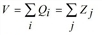
Balancing after trip generation takes place in three steps.
1. Calculation of total production and total attraction for all demand strata except ca.
 ;
; 
2. Calculation of the demand to be compensated of all zones i.
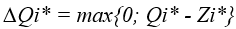 ;
; 
3. Correction of traffic volume in ca, whereby  and
and  are "preliminary" values taken from the formulas in Table 48, Table 49 and Table 50.
If there are non-interchangeable modes, you need to perform the balancing procedure for each of them individually. Then you perform a single balancing procedure for the sum of all interchangeable modes. This, however, is only possible during distribution and mode choice.
The following example will illustrate the method. For simplification it is limited to five demand strata covering all origin-destination types.
|
|
Activity |
Person group |
|||
|
No |
Code |
OD type |
Origin |
Destination |
Origin zone |
|
1 |
HW |
1 |
Home |
Work |
Employees |
|
2 |
HO |
1 |
Home |
Others |
Inhabitants |
|
3 |
WH |
2 |
Work |
Home |
Employees |
|
4 |
OH |
2 |
Others |
Home |
Inhabitants |
|
5 |
OO |
3 |
Others |
Others |
Inhabitants |
|
|
Relevant structural potential |
|||
|
No |
Code |
OD type |
Origin zone |
Destination zone |
|
1 |
HW |
1 |
Like home |
Jobs |
|
2 |
HO |
1 |
Like home |
Jobs in tertiary sector and inhabitants |
|
3 |
WH |
2 |
Jobs |
Like home |
|
4 |
OH |
2 |
Jobs in tertiary sector and inhabitants |
Like home |
|
5 |
OO |
3 |
Jobs in tertiary sector and inhabitants |
Jobs in tertiary sector and inhabitants |
Table 52: Example data for demand strata in an EVA model
The model covers 18 zones, 10 of which belong to the actual study area (type 1) and 8 zones form a cordon around them (type 2). The zones of type 1 feature study area factors of 1.0, those of type 2 of 0.9. The relevant zone attributes are set as follows.
|
Zone |
Type |
Inhabitants |
Employees |
Jobs |
Jobs tertiary |
|
1 |
1 |
7.000 |
3.000 |
2.000 |
1.100 |
|
2 |
1 |
10.500 |
5.500 |
7.000 |
4.500 |
|
3 |
1 |
7.000 |
3.000 |
2.000 |
1.300 |
|
4 |
1 |
5.000 |
2.000 |
1.700 |
1.000 |
|
5 |
1 |
3.000 |
1.200 |
2.500 |
1.600 |
|
6 |
1 |
2.000 |
900 |
1.600 |
1.000 |
|
7 |
1 |
500 |
200 |
2.000 |
1.200 |
|
8 |
1 |
5.000 |
2.000 |
1.000 |
600 |
|
9 |
1 |
7.000 |
3.100 |
2.500 |
1.400 |
|
10 |
1 |
5.000 |
2.000 |
1.500 |
1.000 |
|
11 |
2 |
3.500 |
1.200 |
1.000 |
600 |
|
12 |
2 |
3.000 |
1.100 |
1.000 |
600 |
|
13 |
2 |
2.500 |
1.000 |
1.000 |
600 |
|
14 |
2 |
1.500 |
700 |
500 |
100 |
|
15 |
2 |
1.500 |
600 |
500 |
100 |
|
16 |
2 |
2.000 |
900 |
1.000 |
600 |
|
17 |
2 |
2.000 |
800 |
500 |
300 |
|
18 |
2 |
2.000 |
800 |
500 |
300 |
Table 53: Example data for zone attributes in the EVA demand model (value of the structural properties)
Depending on demand stratum and zone type the following mobility rates are applicable (trips per person in relevant person group).
|
Zone type |
HW |
HO |
WH |
OH |
OO |
|
1 |
0.7800 |
0.9000 |
0.6200 |
0.9000 |
0.6000 |
|
2 |
0.8100 |
0.9000 |
0.6400 |
0.9000 |
0.6000 |
Table 54: Example data for mobility rates in the EVA demand model
The production rates of the structural properties equally depend on demand stratum and zone type.
|
Demand stratum |
Structural property |
Zone type 1 |
Zone type 2 |
|
HW |
|
1.00 |
1.00 |
|
HO |
Inhabitants |
0.50 |
0.50 |
|
Jobs in tertiary sector |
0.50 |
0.50 |
|
|
WH |
|
1.00 |
1.00 |
|
OH |
Inhabitants |
0.50 |
0.50 |
|
Jobs in tertiary sector |
0.50 |
0.50 |
|
|
OO |
Inhabitants |
0.50 |
0.50 |
|
Jobs in tertiary sector |
0.50 |
0.50 |
Table 55: Example data for production rates in the EVA demand model
All demand strata have strong constraints. This results in the productions and attractions of the demand strata displayed in the following tables. The demand strata are based on the formulas in Table 48, Table 49 and Table 50. For clarification the respective step of the calculation process is indicated on top of each column.
- H = Home trips
- Q = Production
- Z = Attraction
- QP = Structural potential origin
- ZP = Structural potential destination
|
Demand stratum |
HW |
||||
|
|
Home |
Origin |
|
Destination |
|
|
Person groups or structural property |
Employees |
Like home |
Jobs |
|
|
|
Calculation step |
1 |
2 |
3 |
4 |
|
|
Zone |
Zone Type |
H |
Q |
ZP |
Z |
|
1 |
1 |
2.340 |
2.340 |
2.000 |
1.578 |
|
2 |
1 |
4.290 |
4.290 |
7.000 |
5.523 |
|
3 |
1 |
2.340 |
2.340 |
2.000 |
1.578 |
|
4 |
1 |
1.560 |
1.560 |
1.700 |
1.341 |
|
5 |
1 |
936 |
936 |
2.500 |
1.972 |
|
6 |
1 |
702 |
702 |
1.600 |
1.262 |
|
7 |
1 |
156 |
156 |
2.000 |
1.578 |
|
8 |
1 |
1.560 |
1.560 |
1,000 |
789 |
|
9 |
1 |
2.418 |
2.418 |
2.500 |
1.972 |
|
10 |
1 |
1.560 |
1.560 |
1.500 |
1.183 |
|
11 |
2 |
875 |
875 |
900 |
710 |
|
12 |
2 |
802 |
802 |
900 |
710 |
|
13 |
2 |
729 |
729 |
900 |
710 |
|
14 |
2 |
510 |
510 |
450 |
355 |
|
15 |
2 |
437 |
437 |
450 |
355 |
|
16 |
2 |
656 |
656 |
900 |
710 |
|
17 |
2 |
583 |
583 |
450 |
355 |
|
18 |
2 |
583 |
583 |
450 |
355 |
|
Total |
|
23.038 |
23.038 |
29.200 |
23.038 |
Table 56: Sample computation of the production and attraction rates for the demand stratum HW
|
Demand stratum |
HO |
||||||
|
|
Home |
Origin |
|
|
|
Destination |
|
|
Person groups or structural property |
Inhab. |
Like home |
Jobs in tertiary sector and inhabitants |
||||
|
Calculation step |
1 |
2 |
3.1 |
3.2 |
4 |
5 |
|
|
Zone |
Zone Type |
H |
Q |
ZP Inh. |
ZP Jobs tert |
ZP Total |
Z |
|
1 |
1 |
6.300 |
6.300 |
3.500 |
550 |
4.050 |
5.796 |
|
2 |
1 |
9.450 |
9.450 |
5.250 |
2.250 |
7.500 |
10.733 |
|
3 |
1 |
6.300 |
6.300 |
3.500 |
650 |
4.150 |
5.939 |
|
4 |
1 |
4.500 |
4.500 |
2.500 |
500 |
3.000 |
4.293 |
|
5 |
1 |
2.700 |
2.700 |
1.500 |
800 |
2.300 |
3.292 |
|
6 |
1 |
1.800 |
1.800 |
1.000 |
500 |
1.500 |
2.147 |
|
7 |
1 |
450 |
450 |
250 |
600 |
850 |
1.216 |
|
8 |
1 |
4.500 |
4.500 |
2.500 |
300 |
2.800 |
4.007 |
|
9 |
1 |
6.300 |
6.300 |
3.500 |
700 |
4.200 |
6.011 |
|
10 |
1 |
4.500 |
4.500 |
2.500 |
500 |
3.000 |
4.293 |
|
11 |
2 |
2.835 |
2.835 |
1.575 |
270 |
1.845 |
2.640 |
|
12 |
2 |
2.430 |
2.430 |
1.350 |
270 |
1.620 |
2.318 |
|
13 |
2 |
2.025 |
2.025 |
1.125 |
270 |
1.395 |
1.996 |
|
14 |
2 |
1.215 |
1.251 |
675 |
45 |
720 |
1.030 |
|
15 |
2 |
1.215 |
1.251 |
675 |
45 |
720 |
1.030 |
|
16 |
2 |
1.620 |
1.620 |
900 |
270 |
1.170 |
1.674 |
|
17 |
2 |
1.620 |
1.620 |
900 |
135 |
1.035 |
1.481 |
|
18 |
2 |
1.620 |
1.620 |
900 |
135 |
1.035 |
1.481 |
|
Total |
|
61.380 |
61.380 |
34.100 |
8.790 |
42.890 |
61.380 |
Table 57: Sample computation of the production and attraction rates for the demand stratum HO
|
Demand stratum |
WH |
||||
|
|
Home |
Destination |
|
Origin |
|
|
Person groups or structural property |
|
Like home |
Jobs |
||
|
Calculation step |
1 |
2 |
3 |
4 |
|
|
Zone |
Zone Type |
H |
Z |
QP |
Q |
|
1 |
1 |
1.860 |
1.860 |
2.000 |
1.253 |
|
2 |
1 |
3.410 |
3.410 |
7.000 |
4.384 |
|
3 |
1 |
1.860 |
1.860 |
2.000 |
1.253 |
|
4 |
1 |
1.240 |
1.240 |
1.700 |
1.065 |
|
5 |
1 |
744 |
744 |
2.500 |
1.566 |
|
6 |
1 |
558 |
558 |
1.600 |
1.002 |
|
7 |
1 |
124 |
124 |
2.000 |
1.253 |
|
8 |
1 |
1.240 |
1.240 |
1.000 |
626 |
|
9 |
1 |
1.922 |
1.922 |
2.500 |
1.566 |
|
10 |
1 |
1.240 |
1.240 |
1.500 |
939 |
|
11 |
2 |
691 |
691 |
900 |
564 |
|
12 |
2 |
634 |
634 |
900 |
564 |
|
13 |
2 |
576 |
576 |
900 |
564 |
|
14 |
2 |
403 |
403 |
450 |
282 |
|
15 |
2 |
346 |
346 |
450 |
282 |
|
16 |
2 |
518 |
518 |
900 |
564 |
|
17 |
2 |
461 |
461 |
450 |
282 |
|
18 |
2 |
461 |
461 |
450 |
282 |
|
Total |
|
18.288 |
18.288 |
29.200 |
18.288 |
Table 58: Sample computation of the production and attraction rates for the demand stratum WH
|
Demand stratum |
OH |
||||||
|
|
Home |
Destination |
|
|
|
Origin |
|
|
Person groups or structural property |
Inhab. |
Like home |
Jobs in tertiary sector and inhabitants |
||||
|
Calculation step |
1 |
2 |
3.1 |
3.2 |
4 |
5 |
|
|
Zone |
Zone Type |
H |
Z |
QP Inh. |
QP Jobs tert |
QP Total |
Q |
|
1 |
1 |
6.300 |
6.300 |
3.500 |
550 |
4.050 |
5.796 |
|
2 |
1 |
9.450 |
9.450 |
5.250 |
2.250 |
7.500 |
10.733 |
|
3 |
1 |
6.300 |
6.300 |
3.500 |
650 |
4.150 |
5.939 |
|
4 |
1 |
4.500 |
4.500 |
2.500 |
500 |
3.000 |
4.293 |
|
5 |
1 |
2.700 |
2.700 |
1.500 |
800 |
2.300 |
3.292 |
|
6 |
1 |
1.800 |
1.800 |
1.000 |
500 |
1.500 |
2.147 |
|
7 |
1 |
450 |
450 |
250 |
600 |
850 |
1.216 |
|
8 |
1 |
4.500 |
4.500 |
2.500 |
300 |
2.800 |
4.007 |
|
9 |
1 |
6.300 |
6.300 |
3.500 |
700 |
4.200 |
6.011 |
|
10 |
1 |
4.500 |
4.500 |
2.500 |
500 |
3.000 |
4.293 |
|
11 |
2 |
2.835 |
2.835 |
1.575 |
270 |
1.845 |
2.640 |
|
12 |
2 |
2.430 |
2.430 |
1.350 |
270 |
1.620 |
2.318 |
|
13 |
2 |
2.025 |
2.025 |
1.125 |
270 |
1.395 |
1.996 |
|
14 |
2 |
1.215 |
1.215 |
675 |
45 |
720 |
1.030 |
|
15 |
2 |
1.215 |
1.215 |
675 |
45 |
720 |
1.030 |
|
16 |
2 |
1.620 |
1.620 |
900 |
270 |
1.170 |
1.674 |
|
17 |
2 |
1.620 |
1.620 |
900 |
135 |
1.035 |
1.481 |
|
18 |
2 |
1.620 |
1.620 |
900 |
135 |
1.035 |
1.481 |
|
Total |
|
61.380 |
61.380 |
34.100 |
8.790 |
42.890 |
61.380 |
Table 59: Sample computation of the production and attraction rates for the demand stratum OH
|
Demand stratum |
OO |
|||||
|
|
Home |
Origin |
|
|
|
|
|
Person groups or structural property |
|
Jobs in tertiary sector and inhabitants |
||||
|
Calculation step |
|
2.1 |
2.2 |
2.3 |
2 |
|
|
Zone |
Zone Type |
H |
QP Inh. |
QP Jobs tert |
QP Total |
Q |
|
1 |
1 |
4.200 |
3.500 |
550 |
4.050 |
3.864 |
|
2 |
1 |
6.300 |
5.250 |
2.250 |
7.500 |
7.156 |
|
3 |
1 |
4.200 |
3.500 |
650 |
4.150 |
3.959 |
|
4 |
1 |
3.000 |
2.500 |
500 |
3.000 |
2.862 |
|
5 |
1 |
1.800 |
1.500 |
800 |
2.300 |
2.194 |
|
6 |
1 |
1.200 |
1.000 |
500 |
1.500 |
1.431 |
|
7 |
1 |
300 |
250 |
600 |
850 |
811 |
|
8 |
1 |
3.000 |
2.500 |
300 |
2.800 |
2.671 |
|
9 |
1 |
4.200 |
3.500 |
700 |
4.200 |
4.007 |
|
10 |
1 |
3.000 |
2.500 |
500 |
3.000 |
2.862 |
|
11 |
2 |
1.890 |
1.575 |
270 |
1.845 |
1.760 |
|
12 |
2 |
1.620 |
1.350 |
270 |
1.620 |
1.546 |
|
13 |
2 |
1.350 |
1,125 |
270 |
1.395 |
1.331 |
|
14 |
2 |
810 |
675 |
45 |
720 |
687 |
|
15 |
2 |
810 |
675 |
45 |
720 |
687 |
|
16 |
2 |
1,080 |
900 |
270 |
1.170 |
1.116 |
|
17 |
2 |
1.080 |
900 |
135 |
1.035 |
987 |
|
18 |
2 |
1.080 |
900 |
135 |
1.035 |
987 |
|
Total |
|
40.920 |
34.100 |
8.790 |
42.890 |
40.920 |
Table 60: Sample computation of the production and attraction rates for the demand stratum OO (1)
|
Demand stratum |
OO |
||||
|
|
Destination |
|
|
|
|
|
Person groups or structural property |
Jobs in tertiary sector and inhabitants |
||||
|
Calculation step |
3.1 |
3.2 |
3.3 |
3 |
|
|
Zone |
Zone Type |
ZP Inh. |
ZP Jobs tert |
ZP Total |
Z |
|
1 |
1 |
3.500 |
550 |
4.050 |
3.864 |
|
2 |
1 |
5.250 |
2.250 |
7.500 |
7.156 |
|
3 |
1 |
3.500 |
650 |
4.150 |
3.959 |
|
4 |
1 |
2.500 |
500 |
3.000 |
2.862 |
|
5 |
1 |
1.500 |
800 |
2.300 |
2.194 |
|
6 |
1 |
1.000 |
500 |
1,500 |
1.431 |
|
7 |
1 |
250 |
600 |
850 |
811 |
|
8 |
1 |
2.500 |
300 |
2.800 |
2.671 |
|
9 |
1 |
3.500 |
700 |
4.200 |
4.007 |
|
10 |
1 |
2.500 |
500 |
3.000 |
2.862 |
|
11 |
2 |
1.575 |
270 |
1.845 |
1.760 |
|
12 |
2 |
1.350 |
270 |
1.620 |
1.546 |
|
13 |
2 |
1.125 |
270 |
1.395 |
1.331 |
|
14 |
2 |
675 |
45 |
720 |
687 |
|
15 |
2 |
675 |
45 |
720 |
687 |
|
16 |
2 |
900 |
270 |
1.170 |
1.116 |
|
17 |
2 |
900 |
135 |
1.035 |
987 |
|
18 |
2 |
900 |
135 |
1.035 |
987 |
|
Total |
|
34.100 |
8.790 |
42.890 |
40.920 |
Table 61: Sample computation of the production and attraction rates for the demand stratum OO (2)
Since all demand strata feature hard constraints, balancing can be performed immediately after trip generation. First of all the total origin and destination traffic of each zone and of the demand strata HW, HO, WH, OW is calculated and the resulting differences are compensated in the OO demand stratum.
|
Note: Note that neither total origin and nor total destination traffic of this demand stratum change. |
|
|
Total HW+HO+WH+OH |
Differences |
||
|
Zone |
Q |
Z |
Q |
Z |
|
1 |
15.689 |
15.534 |
155 |
0 |
|
2 |
28.857 |
29.116 |
0 |
259 |
|
3 |
15.832 |
15.677 |
155 |
0 |
|
4 |
11.418 |
11.375 |
43 |
0 |
|
5 |
8.493 |
8.708 |
0 |
215 |
|
6 |
5.651 |
5.767 |
0 |
116 |
|
7 |
3.075 |
3.368 |
0 |
293 |
|
8 |
10.693 |
10.536 |
157 |
0 |
|
9 |
16.294 |
16.205 |
89 |
0 |
|
10 |
11.293 |
11.217 |
76 |
0 |
|
11 |
6.914 |
6.877 |
37 |
0 |
|
12 |
6.114 |
6.092 |
22 |
0 |
|
13 |
5.314 |
5.307 |
7 |
0 |
|
14 |
3.038 |
3.004 |
34 |
0 |
|
15 |
2.965 |
2.946 |
19 |
0 |
|
16 |
4.514 |
4.523 |
0 |
9 |
|
17 |
3.966 |
3.917 |
49 |
0 |
|
18 |
3.966 |
3.917 |
49 |
0 |
|
Total |
164.086 |
164.086 |
892 |
892 |
Table 62: Sample computation for balancing (1)
|
|
OO before balancing |
OO after balancing |
||
|
Zone |
Q |
Z |
Q |
Z |
|
1 |
3.864 |
3.864 |
3.780 |
3.934 |
|
2 |
7.156 |
7.156 |
7.258 |
7.000 |
|
3 |
3.959 |
3.959 |
3.873 |
4.028 |
|
4 |
2.862 |
2.862 |
2.800 |
2.843 |
|
5 |
2.194 |
2.194 |
2.361 |
2.147 |
|
6 |
1.431 |
1.431 |
1.516 |
1.400 |
|
7 |
811 |
811 |
1.087 |
793 |
|
8 |
2.671 |
2.671 |
2.613 |
2.770 |
|
9 |
4.007 |
4.007 |
3.920 |
4.009 |
|
10 |
2.862 |
2.862 |
2.800 |
2.876 |
|
11 |
1.760 |
1.760 |
1.722 |
1.759 |
|
12 |
1.546 |
1.546 |
1.512 |
1.534 |
|
13 |
1.331 |
1.331 |
1.302 |
1.309 |
|
14 |
687 |
687 |
672 |
706 |
|
15 |
687 |
687 |
672 |
691 |
|
16 |
1.116 |
1.116 |
1.101 |
1.092 |
|
17 |
987 |
987 |
966 |
1.015 |
|
18 |
987 |
987 |
966 |
1.015 |
|
Total |
40.920 |
40.920 |
40.920 |
40.920 |
Table 63: Sample computation for balancing (2)
The results of operation EVA trip generation are stored in zone attributes.
|
Attribute |
Subattribute |
Meaning and range of values |
|
HomeTrips |
Demand stratum |
Home trips for demand stratum Range: floating point number |
|
ProductionsTarget |
Demand stratum |
Productions for demand stratum, before taking account of constraints Range: floating point number |
|
AttractionsTarget |
Demand stratum |
Same for attractions Range: floating point number |
|
Productions |
Demand stratum |
Productions for demand stratum after taking account of constraints and balancing Note This attribute is only available after EVA trip generation if all demand strata feature hard constraints, otherwise after EVA trip distribution / mode choice only. Range: floating point number |
|
Attractions |
Demand stratum |
Same for attractions Range: floating point number |
Table 64: Zone attributes with results of trip generation of the EVA demand model
