Using tour-based calculation, you can save output matrices with different aggregation levels. The demand matrices are calculated from possible combinations of person group, mode, production and attraction activity, and time interval.
Trip distribution: route links through destination choice according to activities
Depending on the destination activity of a trip, the tour-based model assigns it to a destination zone. This destination zone is chosen depending on several factors.
- The utility matrix, which shows the separation from the origin zone (spatially and traffic-wise)
The utility is inversely proportional to impedance values, such as run times or distances, so that the greater the run time or distance to a destination zone, the less its utility.
The utility matrix may also include the logsum of mode-specific utility. In this way, specific skims (e.g. PrT journey time or PuT number of transfers) are included in the total utility with their share in the respective mode.
The utility matrix may also include the logsum. It is composed of the specific utilities of all modes:
Logsum = Utility transformed in Σk of the mode k,
i.e. the natural logarithm of the sum of the transformed mode utilities. The logsum thus simultaneously takes into account mode-specific skims such as the PrT journey time and PuT number of transfers and can thus be interpreted as a general accessibility index.
- The target potential of the zones competing as destinations
- The impact of utility defined via the utility function parameters for each group and each destination activity
These parameters can be estimated beforehand (Estimating gravitation parameters (KALIBRI))
This is how a multitude of trip chains is created through each activity chain. The result of trip distribution is not only a total traffic matrix but also a set of all route chains.
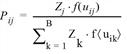
With the destination choice model, the tour-based model needs a target potential Zj for each activity. The target potential specifies the quantitative attractiveness of a zone. This target potential for each zone j, corresponds to the value of the structural property that belongs to the activity (Tour-based model).
The utility function f(uij) is pivotal in the destination choice model. It specifies the probability Pij with which one of the zones j is selected as destination zone (from all destination alternatives) of origin zone i.

where
|
Fij |
Number of trips from zone i to zone j |
|
Qi |
Productions in zone i |
|
Pij |
Choice probability of destination j for origin zone i |
|
Zj |
Target potential in zone j |
|
k |
Index of zones (with k = the smallest zone number and B = the number of zones) |
whereby uij describes the utility relation ij and the utility function f(uj)) (e.g. of the type Logit) can consequently be defined as  . All other weighting functions of the EVA demand model can also be used as utility functions in the tour-based model (EVA trip distribution and mode choice).
In this case, the choice of the parameter c for each activity plays the decisive role in the destination choice. c expresses the influence of the utility over the destinations of the activity. If c = 0, then the utility uij has no influence on the choice of destination. The larger c is, the larger is the impact of utility uij on the choice of the destination (Gravity model calculation).
Separate function parameters are defined for each combination of group of persons and target activity.
To give you a better idea of what the three main model elements of destination choice, namely destination potential, utility function and utility matrix stand for, we will continue with the example we used for trip generation (Example of trip generation with the tour-based model).
Example of trip distribution
A Logit utility function ( with parameter c = 0.4) is used to represent the changeovers from and to the individual activities.
The 93.4 trips of the activity pattern HW have to lead from the origin (zone 1) to the potential destination zones, containing jobs. The tour-based model distributes these 93.4 trips to the destination zones, according to the previously described destination choice model.
To make it easier, let us assume that zone 2 is the only zone with jobs, which therefore has a positive destination potential for the activity work. Expressed in numbers this would be approximately Z1 = 0, Z2 = 100, Z3 = 0. The tour-based trip distribution formulas produce the following results P11 = 0, P12 = 1 and P13 = 0, and therefore F11 = 0, F12 = 93.4 and F13 = 0. Zone 2 is therefore the destination of all trips of zone 1.
|
Note: The definition of the utility function in this case does not influence the calculation. |
After the activity work, based on zone 2, the probability for the choice of shopping destinations is calculated for the subsequent trips WO. It is assumed, that the destination potentials for the activity "Shopping" are defined as follows: Z1 = 0, Z2 = 50, Z3 = 50. Based on travel times and distances, the utility defined for changeover WO, with the relation 2-2, is twice as high as the changeover with the relation 2-3, thus approximately u22 = 2 and u23 = 1. The tour-based trip distribution formulas produce the following results P21 = 0, P22≈ 0.6 and P23≈ 0.4, and therefore F21 = 0, F22≈ 56.0 and F23≈ 37.4. 40 % of the trips thus lead to zone 3 and 60 % to zone 2 (i.e. trips within the cell).
Here, multiplication of the destination probability of the work and shopping destinations takes place in the system.
For the last activity pair of the chain, namely PH, destination choice is no longer necessary, because zone 1 as a residential district and origin of the first trip of the chain, is also the destination of the last trip of the chain.
This results in the following transition matrices.
- Matrix F1 for the first activity transfer (Destination activity W)
|
Zone |
93.4 |
1 |
2 |
3 |
|
93.4 |
Total |
0 |
93.4 |
0 |
|
1 |
93.4 |
0 |
93.4 |
0 |
|
2 |
0 |
0 |
0 |
0 |
|
3 |
0 |
0 |
0 |
0 |
- Matrix F2 for the second activity transfer (Destination activity O)
|
Zone |
93.4 |
1 |
2 |
3 |
|
93.4 |
Total |
0 |
56.0 |
37.4 |
|
1 |
0 |
0 |
0 |
0 |
|
2 |
93.4 |
0 |
56.0 |
37.4 |
|
3 |
0 |
0 |
0 |
0 |
- Matrix F3 for the third activity transfer (Destination activity H)
|
Zone |
93.4 |
1 |
2 |
3 |
|
93.4 |
Total |
93.4 |
0 |
0 |
|
1 |
0 |
0 |
0 |
0 |
|
2 |
56.0 |
56.0 |
0 |
0 |
|
3 |
37.4 |
37.4 |
0 |
0 |
Summed up, the following total demand matrix applies FG.
|
Zone |
280.2 |
1 |
2 |
3 |
|
280.2 |
Total |
93.4 |
149.4 |
37.4 |
|
1 |
93.4 |
0 |
93.4 |
0 |
|
2 |
149.4 |
56.0 |
56.0 |
37.4 |
|
3 |
37.4 |
37.4 |
0 |
0 |
Summary of this destination choice example
- HW: 100 % leave zone 1 with destination zone 2
- WO: 60 % remain in zone 2 and 40 % leave zone 2 to zone 3
- OH: 100 % return to zone 1.
The corresponding route chains are as follows:
- 1-2-2-1: 93.4 • 100 % • 60 % • 100 % = 56.0
- 1-2-3-1: 93.4 • 100 % • 40 % • 100 % = 37.4
The following route chains have been created:
- 56.0 route chains 1-2-2-1
- 37.4 route chains 1-2-3-1
|
Notes: The following behavioral aspects should be taken into consideration when you define the utility parameters.
|
The tour-based model allows specific utility matrices to be imported for each activity. Combinations of distances and journey times can be used as a basic parameter in utility matrices.
|
Note: The absolute value of a destination potential is first of all irrelevant, because it only flows into the destination choice model comparatively to the sum of destination potentials of all zones. Destination potential " jobs = 1,000" for a zone does not necessarily mean that the tour-based model produces 1,000 trips for destination activity work. In fact, the destination traffic depends on the product of destination potential and utility function value in relation to the other zones. |
If, however, the absolute value of the destination potential of an activity is very important, as for example for the number of jobs, this can flow into the calculation via the Destination-sided attraction option. If there are approx. 6,000 jobs in the study area, 1,000 jobs mean there is a relative destination potential of 1,000/6,000 = 1/6 for the activity work. If a demand stratum has a total of 3,000 home trips, the absolute zone destination potential standardized to the total of home trips for this demand stratum is 3 • 1/6 = 500. This absolute value for the demand stratum is used as a constraint in the doubly-constrained gravity model (Gravity model calculation).
In general, this preset distribution of destination potential for individual demand strata does not correspond to reality. In fact, for destination-bound binding, the destination potential of all demand strata is utilized together. A calculation performed across all demand strata allows for distribution of the destination potential across all demand strata, producing one result. The examination of individual demand strata is based on the assumption of a preset distribution.
You can save your trip distribution results in an aggregated form to total demand matrices per person group as well as per combination of time interval, mode, origin and destination activity.
Mode choice: discrete distribution model
The tour-based demand model has a behavior-oriented concept, which models the following aspects of the decision-making of road users.
- The socioeconomic position and the mode availability of the person making the decision (by differentiating according to person groups)
- Different attributes of all modes (through the utility model)
- Freedom of choice restrictions within trip chains (by definition of exchangeable and non-exchangeable modes)
This decision problem is illustrated in a discrete distribution model, which specifies the probability for mode choice in every available route link.
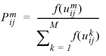
To do so, the subjective utility has to be calculated in dependency of the mode skims (in-vehicle time, access and egress times, fare, etc.). If required, you can define several utilities per destination activity.
This model has the following functional form.
where
|
i, j |
Indices of the traffic zones |
|
m |
Index of modes (M = total number) |
|
Pmij |
Probability of selecting mode m for trip from i to j |
|
umij |
Utility when choosing mode m for trip from i to j |
The utility function  can for example be a Logit utility function and thus be defined as
  As an alternative, all available types of evaluation functions can be used from the EVA demand method as a utility function for the tour-based mode choice (EVA trip distribution and mode choice).
As a base parameter for the utility matrices any distance combinations and mode specific skims can be used, such as travel times, access and egress times, and fares.
The nested Logit model is a special variant for which mode choice is nested using the Logit approach. For this purpose, a decision tree is defined that shows the hierarchical structure of the model. The decision tree may look as follows:
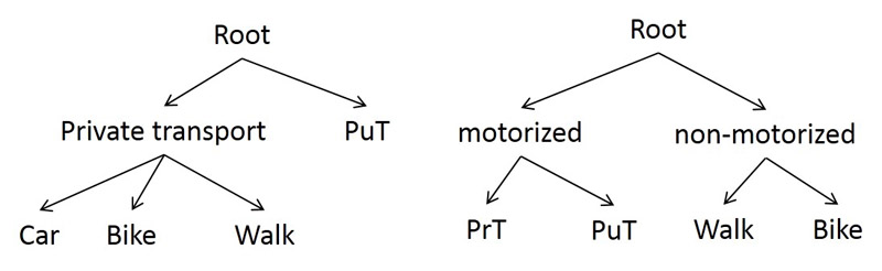
Under the root node, nested nodes (such as "private transport", "motorized", "non-motorized") or mode nodes (such as "car", "bike", "walk") can be defined. There must be at least one mode node for each mode of a demand model. Any nesting depth can be used if each mode is only used once in the decision tree. If a mode is used multiple times in a decision tree, the nesting depth is limited to two levels under the root node and calculations are based on the cross-nested Logit model.
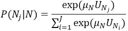
For the nested Logit model, the probabilities of mode choice are calculated as follows:
Let us assume there is a node N with a number of child nodes (mode nodes or nested nodes) N1,…,NJ. The utility of each node Nj is specified as UNj, and the scaling parameter at node N is μN. Then child node Nj is selected with the following probability:
The utility in the utility definition of the node is called VN.
- If N is a mode node on the bottom level, then UN=VN.
- Otherwise, N1,...,Nj are the child nodes of nested node N. The scaling parameter of N is μN. The utility UN of a node N is calculated from:
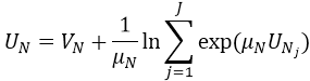 the summand on the right called LogSum
The probability of selecting a mode node results from the product of probabilities of the hierarchy levels of the respective branch. The parent node of a node N is specified as parent(N). N is a mode node. For a k∈N, the parentk(N) is the root node of the decision tree. The the probability of selecting mode node N results from:

If a mode is defined multiple times in the decision tree, calculations are based on the cross-nested Logit model (Abbe, Bierlaire, Toledo, 2007, pp. 795-808).
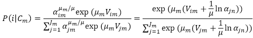
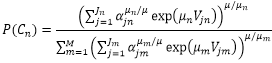
We assume that under the root node there are many nested nodes C1,…,CM, and in each nest Cm, there are a lot of mode nodes N1m,…, . Each mode node Njm is assigned an allocatin parameter αjm≥0. The scaling parameter of the root node is specified as μ, the scaling parameter of a nest node Cm is specified as μm. Finally, Vjm and Vm are the utilities of the utility definition of mode node Njm or nested node Cm.
The probability of selecting a mode node Nim, given nested node Cm was selected, is calculated with the following formula:
 .
.
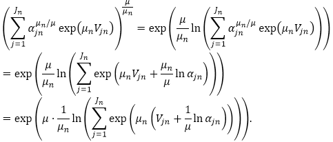
If the utility of nested node Cm is null, i.e. Vm=0, then the probability of selecting a nested node Cm is:
This means
Last but not least, we would like to explain the importance of the route chain concept for mode choice.
In Visum the modes are divided into the following groups:
- exchangeable modes (generally walk, passenger and public transport)
- non-exchangeable modes (car, bike)
The tour-based model calculates a discrete distribution model (for example Logit) when first calculating the trip of each route link (for a person group) and chooses one from all modes. If the first mode is a non-exchangeable mode, the entire trip chain is maintained independent of the attributes of this mode of the successive trip. If an exchangeable mode was selected for the first trip, mode choice is carried out for the remaining chain trips, however, only within the exchangeable modes.
Example of mode choice
We will continue with the example from the trip distribution (Example of trip distribution) and will determine the matrices for each activity transfer for the three modes Car (C), PuT (X) and Walk (W). Only mode P cannot be exchanged. The set of exchangeable modes X and W in short is also designated with A. A Logit utility function is used again to represent the changeovers from and to the individual activities,
i.e. , using the parameter c = 0.4. The utility matrices um for each mode m are provided by
- uC
|
Zone |
1 |
2 |
3 |
|
1 |
3 |
3 |
3 |
|
2 |
3 |
3 |
3 |
|
3 |
3 |
3 |
3 |
- uX
|
Zone |
1 |
2 |
3 |
|
1 |
2 |
1 |
1 |
|
2 |
1 |
2 |
2 |
|
3 |
1 |
2 |
2 |
- uW
|
Zone |
1 |
2 |
3 |
|
1 |
1 |
1 |
1 |
|
2 |
1 |
1 |
1 |
|
3 |
1 |
1 |
1 |
After analyzing the formula above, the following probability matrices apply.
- PC
|
Zone |
1 |
2 |
3 |
|
1 |
0.472 |
0.526 |
0.526 |
|
2 |
0.526 |
0.472 |
0.472 |
|
3 |
0.526 |
0.472 |
0.472 |
- PX
|
Zone |
1 |
2 |
3 |
|
1 |
0.316 |
0.237 |
0.237 |
|
2 |
0.237 |
0.316 |
0.316 |
|
3 |
0.237 |
0.316 |
0.316 |
- PW
|
Zone |
1 |
2 |
3 |
|
1 |
0.212 |
0.237 |
0.237 |
|
2 |
0.237 |
0.212 |
0.212 |
|
3 |
0.237 |
0.212 |
0.212 |
- PA = PX + PW
|
Zone |
1 |
2 |
3 |
|
1 |
0.528 |
0.474 |
0.474 |
|
2 |
0.474 |
0.528 |
0.528 |
|
3 |
0.474 |
0.528 |
0.528 |
Interesting are also the probabilities for modes X and W within the exchangeable modes.
- PAX = PX / PA
|
Zone |
1 |
2 |
3 |
|
1 |
0.598 |
0.5 |
0.5 |
|
2 |
0.5 |
0.598 |
0.598 |
|
3 |
0.5 |
0.598 |
0.598 |
- PAW = PW / PA
|
Zone |
1 |
2 |
3 |
|
1 |
0.402 |
0.5 |
0.5 |
|
2 |
0.5 |
0.402 |
0.402 |
|
3 |
0.5 |
0.402 |
0.402 |
The matrix of the first non-exchangeable mode Car for all activity transfers is calculated. The matrix for the first activity transfer is the product of PC with the total demand matrix F1 of the first transfer.
- Total demand matrix F1 for the first activity transfer (Destination activity W)
|
Zone |
93.4 |
1 |
2 |
3 |
|
93.4 |
Total |
0 |
93.4 |
0 |
|
1 |
93.4 |
0 |
93.4 |
0 |
|
2 |
0 |
0 |
0 |
0 |
|
3 |
0 |
0 |
0 |
0 |
- Matrix FP1 for mode C and the first activity transfer (destination activity A)
|
Zone |
49.12 |
1 |
2 |
3 |
|
49.12 |
Total |
0 |
49.12 |
0 |
|
1 |
49.12 |
0 |
49.12 |
0 |
|
2 |
0 |
0 |
0 |
0 |
|
3 |
0 |
0 |
0 |
0 |
With the next activity changeover, these 49.12 trips will be distributed across zones 2 and 3 according to the distribution probabilities (P22 = 0.6 or P23 = 0.4).
- Matrix FC2 for mode C and the second activity transfer (Destination activity O)
|
Zone |
49.12 |
1 |
2 |
3 |
|
49.12 |
Total |
0 |
29.47 |
19.65 |
|
1 |
0 |
0 |
0 |
0 |
|
2 |
49.12 |
0 |
29.47 |
19.65 |
|
3 |
10 |
0 |
0 |
0 |
Finally, the trips have to end back at the last activity transfer in their origin zone 1.
- Matrix FC3 for mode C and the third activity transfer (Destination activity H)
|
Zone |
49.12 |
1 |
2 |
3 |
|
49.12 |
Total |
49.12 |
0 |
0 |
|
1 |
0 |
0 |
0 |
0 |
|
2 |
29.47 |
29.47 |
0 |
0 |
|
3 |
19.65 |
19.65 |
0 |
0 |
Summed up, the following Car total demand matrix applies: FCT
|
Zone |
147.36 |
1 |
2 |
3 |
|
147.36 |
Total |
49.12 |
88.59 |
19.65 |
|
1 |
49.12 |
0 |
49.12 |
0 |
|
2 |
88.59 |
29.47 |
29.47 |
19.65 |
|
3 |
19.65 |
19.65 |
0 |
0 |
To determine the total demand matrix for non-exchangeable modes, this Car matrix is subtracted from the total demand matrix FT (from trip distribution).
- FT
|
Zone |
280.2 |
1 |
2 |
3 |
|
280.2 |
Total |
93.4 |
149.4 |
37.4 |
|
1 |
93.4 |
0 |
93.4 |
0 |
|
2 |
149.4 |
56.0 |
56.0 |
37.4 |
|
3 |
37.4 |
37.4 |
0 |
0 |
The difference first results in the total demand matrix for all non-exchangeable modes.
- FA
|
Zone |
132.84 |
1 |
2 |
3 |
|
132.84 |
Total |
44.28 |
70.81 |
17.75 |
|
1 |
44.28 |
0 |
44.28 |
0 |
|
2 |
70.81 |
26.53 |
26.53 |
17.75 |
|
3 |
17.75 |
17.75 |
0 |
0 |
For this matrix mode choice now takes place within the exchangeable modes PuT and Walk, to obtain the total demand matrices for modes PuT and Walk. The matrix is multiplied with the probabilities PAX and PAW.
- PuT total demand matrix FX
|
Zone |
70.75 |
1 |
2 |
3 |
|
70.75 |
Total |
22.14 |
38.00 |
10.61 |
|
1 |
22.14 |
0 |
22.14 |
0 |
|
2 |
39.74 |
13.27 |
15.86 |
10.61 |
|
3 |
8.87 |
8.87 |
0 |
0 |
- Walk total demand matrix FW
|
Zone |
62.09 |
1 |
2 |
3 |
|
62.09 |
Total |
22.14 |
32.81 |
7.14 |
|
1 |
22.14 |
0 |
22.14 |
0 |
|
2 |
31.07 |
13.26 |
10.67 |
7.14 |
|
3 |
8.88 |
8.88 |
0 |
0 |
Make sure that the Car total demand matrix has identical row and column sums for each zone, whereas this is not mandatory for the PuT and Walk matrices.
The mode choice results are saved in an aggregated form to demand matrices per person group and mode. In addition, you can limit the usage of time interval and origin and destination activity data for matrices with disaggregated data.
