Signalized nodes

Notes: Signalized nodes are described in the HCM 2000, in chapter 16. In the HCM 2010, they are described in chapters 18 and 31, and in the HCM 6th Edition and HCM 7th Edition, in chapters 19 and 31. Instead of the method described here for signalized nodes, the method for yield-controlled nodes is applied to nodes and main nodes of the signalized control type, to which no has been allocated or whose signal controller has been turned off.

The basic flow chart for performing capacity analyses for signalized intersections is displayed in Image 74. You input the intersection geometry, volumes (counts or adjusted demand model volumes), and signal timing. The intersection geometry is deconstructed into lane (or signal) groups, which are the basic unit of analysis in the HCM method.

A lane (or signal) group is a group of one or more lanes on an intersection approach having the same green stage. If, for example, an approach has just one pocketed exclusive left turn and one shared through and right turn, then there are usually two lane groups – the left and the shared through/right.

Note: According to HCM 2010 and later editions, lane allocation follows different rules. Here, shared lanes always form a separate lane group. A more detailed description can be found in the HCM 2010, on pages 18-33 and in the HCM 6th Edition as well as HCM 7th Edition, on pages 19-43.

The volumes are then adjusted via peak hour factors, etc. For each lane group, the saturation flow rate (SFR), or capacity, is calculated based on the number of lanes and various adjustment factors such as lane widths, signal timing, and pedestrian volumes. Having calculated the demand and the capacity for each lane group, various performance measures can be calculated. These include, for example, the v/c ratio, the average amount of control delay by vehicle, the Level of Service, and the queues.

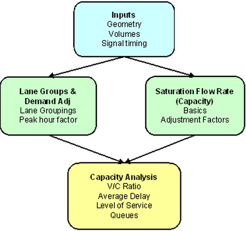
Image 74: Capacity analysis process for signalized nodes

Note: A corresponding flow diagram can be found in the HCM 2010, on pages 18-32 and in the HCM 6th Edition as well as HCM 7th Edition on pages 19-42..

If you use the operations model for signalized nodes, the Visum attributes in Table 100 will show effect. Note that some attributes are only considered from a certain HCM version. Make sure that they are set to realistic values prior to running the analysis.

Alternatively to the calculation method according to HCM, you can apply one of the following methods:

• ICU1
• ICU2
• Circular 212 Planning
• Circular 212 Operations

From the HCM, these procedures differ in just three aspects:

• Definition of the ideal saturation flow rate
• Calculation of the final saturation v/s (volume/saturation flow rate) for the node
• Determination of the Level of Service (LOS)

Steps Step 6, Step 9, and Step 13 below describe the calculation variants in detail.

Note: Visum allows for control access to RBC and Vissig controllers. Vissig controllers provide fixed-time control strategies. RBC controllers provide pre-timed or actuated control strategies (also fully or semi-actuated). HCM 2010 provides a computation method for fixed-time strategies and for traffic-actuated strategies as well. Visum uses fixed-time strategies for Vissig controllers. The strategy used for RBC controllers depends on the type of traffic actuation. This method is described in the HCM 2010, in chapters 18 and 31, and in the HCM 6th Edition, in chapters 19 and 31. Prior to the computation, Visum imports the signal control data for the control strategy from the corresponding control file.

Network object	Attribute	Description / Effect
Link	ICA arrival type	Level of platooning in traffic arriving at the ToNode, subsequently used in steps Step 10 + Step 14a
Link	Share of HGV	Proportion of heavy goods vehicles, used in step 6b. One value applies to all turns originating from the link.
Link	Space per PCU	Used in Step 6 for calculation of the number of vehicles that fit on a pocket lane.
Link	Slope	Used in Step 6
Link	ICA is work zone in approach	Indicates a temporary construction site in the access area of the intersection, used in step 6 (from HCM 6th Edition).
Link	ICA number of open lanes in work zone	Number of lanes open during temporary construction, used in step 6.
Link	ICA lane width in work zone	Total width of lanes open during temporary construction, used in step 6.
Link	ICA sustained spillback factor	Used in step 6.
Link	ICA downstream lane blockage factor	Used in step 6.
Link	ICA right turn will influence opposing left turn	The time gap choice of right turns (right-hand traffic) is influenced by left turns of the opposite approach, even if they have their own lanes, used in step 6.
Node	ICA peak hour factor volume adjustment	Factor for adjustment of initial volumes to peak volumes. Volumes are divided by both node and turn adjustment factors.
Node	ICA loss time	Used in Step 9. Only required for SG-based signal control. For other types of signal control the value is inferred automatically.
Node	ICA use preset loss time	Decides whether the node attribute ICALossTime or an automatically calculated value is to be used for loss time computation in step Step 9.
Node	ICA is central business district	Is the node located in the Central Business District?; used in step 6e.
Node	ICA sneakers	Number of vehicles which can line up in the node area during a cycle. The value in [veh] applies to all movements at the node The cycle time is used for the minimum capacity calculation for each movement.
Node	SC number	Points to the signal controller.
Node	ICAShareCAVs	Optional consideration of the share of autonomous vehicles. The value range is between 0 and 100%. The attribute is considered for the calculation of the ideal saturation flow rate in step 6 starting with the HCM 7th Edition.
Geometry	All	Geometry data of lanes, lane turns and crosswalks.
Turn	ICAPHFVolAdj	Initial volume adjustment to peak period; volumes are divided by both node and turn adjustment factors
Turn	ICA Preset saturation flow rate	Overwrites optionally the global saturation flow rate in the procedure parameters. Can be overwritten by the specific lane value of this attribute, if applicable.
Turn	ICA upstream adjustment	Adjustment factor for upstream filtering / metering, used in steps Step 10b +Step 14b
Turns	Share of HGV	Proportion of heavy goods vehicles, used in step 6b. Fixed value that refers to turns.
Turns	ICA delay of unsignalized movement	Waiting time for unsignalized movement, used in steps 11 and 12.
Signal control	All	Definition of signal groups, stages (where applicable), and signal timing.
Signal controller	Used intergreen method	Is used in Step 9 for loss time calculation.
Signal controller	Turned off	If a signal controller is marked as 'turned off', the node will be calculated according to the „yield control“ control type.
Signal group	ICA loss time adjustment	Is added to the actual green time. The actual green time and ICA loss time adjustment sum up to the green time on which all computations are based.
Signal group	ICA start-up loss time	Affects calculation of effective green time according to HCM formulae.
Leg	ICA Local bus stopping rate	Number of stops in Veh/h, used to calculate the adjustment factor for the saturation flow rate in order to account for bus stops according to HCM formula.
Leg	Has on-street parking on right/left	Describes whether parking is allowed on the right or left side of the street, is used to calculate the adjustment factor of the saturation flow rate in order to account for parking according to the HCM formula.
Leg	On-street parking maneuver rate right/left	Number of parking maneuvers / h on the right or left side of the street, is used to calculate the adjustment factor of the saturation flow rate in order to account for parking according to the HCM formulae.
Leg	ICA bicycle volume	Number of bicyclists per hour for the determination of the adjustment factor for the saturation flow rate.
Lanes	Number of vehicles	User-defined number of vehicles ≥ 0.0 the pocket accommodates. This attribute is only regarded if the attribute Use number of vehicles is true and if the global procedure parameter 'Regard pocket length for saturation flow rate calculation' is active.
Lanes	Use number of vehicles	Decision, whether Number of vehicles of the lane shall be used. If this attribute is not true, the number of vehicles is determined from the pocket length and the attribute Space per PCU.
Lanes	Length	Lane length if pockets are concerned. This attribute is only regarded if the attribute Use number of vehicles is not true and if the global procedure parameter 'Regard pocket length for saturation flow rate calculation' is active. The number of vehicles is calculated from the length of the pocket and the attribute Space per PCU.
Lanes	Width	Width of the lane. On this basis, the saturation flow rate is calculated for the lane group to which the lane belongs. The calculated lane group width is the mean value derived from the width values of all lanes of this group.
Lanes	ICA Preset saturation flow rate	Saturation flow rate for the lane after consideration of all adjustment factors. Use this attribute to set the saturation flow rate directly if the HCM-based adjustment factors do not reflect the actual circumstances of the lane. This value overwrites the procedure parameter value and also turn-related values, if applicable.
Lanes	ICA Use preset saturation flow rate	Decision, whether the internally calculated saturation flow rate shall be replaced by the ICA Preset saturation flow rate value.
Lanes	ICA user-defined utilization share	Utilization share of the lane within a multi-lane group. The sum of the input shares is automatically scaled to 100%, thus you can enter relative weights per lane. This value is used in step Step 6.
Lanes	ICA use user-defined utilization share	Decision, whether the internally calculated utilization share shall be replaced by the ICA user-defined utilization share value.
Crosswalk	Pedestrian volume	Number of pedestrians per hour for the determination of the adjustment factor for the saturation flow rate.

Table 100: Input attributes for signalized nodes

Note: The link attribute Turn on red is not regarded for calculation.

Output is possible through the attributes listed in Table 101.

Network object	Attribute	Description / Effect
Node	Turn tCur maximum Turn tCur mean Turn tCur total	Sum, average, max of turn tCur. Now obsolete, since available as indirect attributes, but retained for backward compatibility.
Node	Design volume capacity ratio PrT	The volume/capacity ratio based on the design volume
Node	Design volume PrT [veh]	The volume in [veh/h] passed into the HCM calculation, as defined in the procedure parameters
Node	Design volume PrT [PCU]	The volume in [PCU/h] passed into the HCM calculation, as defined in the procedure parameters
Node	Level of service
Node	Level of service mean delay
Turn	Design volume PrT [veh] ...	The volume in [veh/h] passed into the HCM calculation, as defined in the procedure parameters
Turn	Design volume PrT [PCU]...	The volume in [PCU/h] passed into the HCM calculation, as defined in the procedure parameters
Turn	ICA final volume	After all adjustments
Turn	ICA final capacity	Effective capacity, taking into account all opposing traffic etc.
Turn	ICA calculated saturation flow rate	After all adjustments
Turn	ICA average back of queue	Average queue length
Turn	ICA back of queue for defined percentile	Percentile of queue length. Specify in the procedure parameters which percentile is calculated.
Turn	Level of service	Level of service of the turn
Turn	tCur-PrTSys	TSys-specific travel time tCur in loaded network

Table 101: Output attributes for signalized nodes

Step 1: Lane volume calculation based on movement volumes

This step distributes the movement volumes to lanes according to the user-defined geometry. The basic distribution rule is to distribute the volumes uniformly to the lanes while taking the input movement volumes into account. The implemented method is the same as in the all-way stop method (All-way stop). You can overwrite a lane's utilization share within its lane group, if applicable (lane attribute ICA user-defined utilization share).

Here, HCM 2010 and HCM 2000 differ significantly. According to HCM 2010, the calculation is much more complex. In HCM 2010, lane volume calculation is an iterative process taking the saturation flow rates into account. For a description, please refer to HCM 2010, pages 31-30 to 31-37.

Step 2: Volume adjustments by means of peak hour factors

The input lane volumes are adjusted to represent the peak hour volumes through the peak hour factor (phf). The phf is defined as:

vi = vg / PHF

where

vi	adjusted volume for lane groupi
vg	unadjusted (input) volume for lane group g
PHF	Peak hour factor (0, 25 - 1,0)

Step 3: Calculation of de facto lane groups left/though/right

De facto lane groups are shared lanes with 100% of their volume making one movement. If, for example, a lane group is a shared left and through lane, and 100% of the lane volume is making a left movement, then the lane group is converted to a de facto exclusive left lane group.

In the HCM 2010, the set of lane groups is not affected by the volumes of turning movements. As described above, shared lanes always form a lane group of its own, even if only a single turning direction is used actually.

Step 4: Calculation of the types of left turns

The type of left turn needs to be determined in order to calculate the left turn adjustment factor. The left turn type is set as follows:

• Fully controlled if all turns of an approach are conflict free during their green times.
• Fully secured if the left turns are conflict free during green time.
• Fully secured + permitted if during green time left turns are first fully secured and then permitted.
• Permitted + fully secured if during green time left turns are first permitted and then fully secured.
• Without left turn stage, all other cases.

Step 5: Proportions of left turning and right turning vehicles calculation by lane group

The proportion of right and left turn volume by lane group needs to be calculated.

PLT = vLT / vi

PRT = vRT / vi

where

PLT	proportion left turn volume by lane group
PRT	proportion right turn volume by lane group
vi	adjusted volume by lane group
vLT	volume of left turning vehicles by lane group
vRT	volume of right turning vehicles by lane group

In HCM 2010, the iterative method mentioned in Step 1 is used for the calculation of the turning movement proportions on shared lanes. For the description in detail, please refer to HCM 2010, page 31-30 et seqq.

Step 6: Saturation flow rate calculation by lane group

The saturation flow rate is the amount of traffic that can make the movement under the prevailing geometric and signal timing conditions. The saturation flow rate starts with an optimum capacity, which is usually is 1,900 vehicles per hour, per lane (vphpl), according to HCM 2000 and HCM 2010.

From HCM 7, the share of autonomous vehicles (CAV) at the node is taken into account when calculating the ideal saturation flow rate per lane.

For calculation variants ICU1 and ICU2, however, the ideal saturation flow rate is 1,600 vehicles per hour, per lane. For the Circular 212 variant, it is taken from the table below:

Method	2 stages	3 stages	4+ stages
Planning	1,500	1,425	1,375
Operations	1,800	1,720	1,650

This number decreases due to various factors. The SFR is defined as:

si = (so)(N) • (fw)(fHV)(fg)(fp)(fa)(fbb)(fLu)(fRT)(fLT)(fLpb)(fRpb)(fWZ)(fms)(fsp)

where

si	saturation flow rate of lane group i
so	ideal saturation flow rate per lane (generally 1,900 vphpl)
N	Number of lanes in lane group
fw	factor for lane width adjustment
fHV	HGV adjustment factor (*)
fg	adjustment factor for approach grade (*)
fp	adjustment factor for parking
fa	adjustment factor for the position of the link to city center (CBD true/false)
fbb	adjustment factor for bus stop blocking
fLu	adjustment factor for lane usage
fRT	adjustment factor for right turns
fLT	adjustment factor for left turns (***)
fLpb	adjustment factor for pedestrians and bicyclists on left turns
fRpb	adjustment factor for pedestrians and bicyclists on right turns
fWZ	adjustment factor for work zones (**)
fms	adjustment factor for lane blocking (**)
fsp	adjustment factor for persistent spillback (**)

(*) The adjustment factors for trucks and slopes were combined in the HCM 6th Edition and replace the previously separate factors for trucks and slopes in the HCM 2000 and 2010.

(**) HCM 6th Edition and higher.

(***) as of HCM 7th edition, the share of autonomous vehicles at the node is additionally taken into account.

First the description of the main calculation is described and then the various SFR adjustment factors are calculated.

If an ICAIdealSatFlowRate is specified for a turn, it will replace the final result of Step 5. All adjustment calculations are then bypassed.

The calculations according to HCM 2000 or HCM 2010 are similar. The set of factors taking effect on the saturation flow rate is the same. Merely the calculations of the factors fw (HCM 2010, page 18-36), fLpb and fRpb differ. The latter are calculated by means of the iterative method, which is described in HCM 2010, pages 31-30 to 31-37.

For the calculation listed in the HCM 6th Edition, the adjustment factors for trucks and slopes were combined. In addition, a new adjustment factor was introduced that accounts for construction work on an approach. The adjustment factors for persistent spillback and lane blocking are also considered. The entire formula for calculating the saturation flow rate is listed in the HCM 6th Edition, on pages 19-44.

Deviating from HCM 2000 , the ideal saturation flow rate so of pocket lanes can also be calculated by the number of vehicles which can be accommodated there. The number n of vehicles can be set by lane. Alternatively, it results from the division of the pocket lane length by the standard vehicle length which is set by link.

The alternative calculation method using lane length data is only applied if the lane group consists of one or more straight through lane(s) and exactly one pocket lane. The pocket lane must be of a straight through lane or a through-left type or a through-right type lane. If these conditions are not satisfied, the regular HCM calculation method will be applied.

The optimal saturation flow rate so of a two-lane group, which consists of a through lane and a pocket, where there is space for n vehicles, then is as follows:

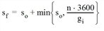
Here, so is the ideal saturation flow rate, n is the number of vehicles which can be accommodated on the pocket, gi is the effective green time and sf is the resulting saturation flow rate of the lane group.

For shared lanes, the calculation is more complex. Taking a through lane with only straight turns and a shared left/straight pocket, then the resulting saturation flow rate sf is as follows:

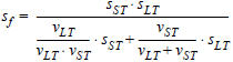
Here, vLT and vST are the volumes of the left and the straight turns, sLT is the ideal saturation flow rate of the left turn - therefore 1,900 vphpl - and sST is the ideal saturation flow rate of the through lanes which results from the first equation.

Step 7: Calculation of actual green times

The effective green time (or actual green time for a lane group) needs to be calculated next. The effective green time results as follows:

gi = Gi + li

where

gi	effective green time per lane group
Gi	green time per lane group
li	loss time adjustment per signal group

Step 8: Capacity calculation per lane group

Related to the SFR is the capacity. The saturation flow rate is the capacity if the movement has 100 % of the green time (this means, the signal controller is always green for the movement). The capacity, however, accounts for the fact that the movement must share the signal controller with the other movements at the intersection, and therefore scales the SFR by the percent of green time in the cycle. The capacity of a lane group is then defined as follows:

ci = si • (gi / C)

where

ci	capacity i
si	saturation flow rate i
C	cycle time
gi / C	green ratio i

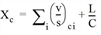
Step 9: Calculation of the critical vol/cap ratio for the entire intersection

The critical v/c ratio of nodes is defined below. The HCM method is concerned with the critical lane group for each signal stage. The critical lane group is the lane group with the largest volume/capacity ratio unless there are overlapping stages. If there are overlapping stages, then the maximum of the different combinations of the stages is taken as the max. For the description of this method, please refer to HCM 2000, page 16-14, or HCM 2010, page 18-41.

Only if the intergreen method Amber and Allred is used for the signal control, loss times will be determined at all. Per signal group, the loss time results from the amber time and allred time total minus loss time adjustment.

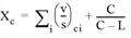
where

Xc	critical saturation (v/c ratio) per intersection
	volume/capacity ratios for all critical lane groups
C	cycle time
L	loss time total of the signal groups of all critical lane groups

Below is an example calculation of critical lane group per signal stage with overlap.

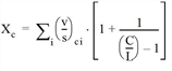
For computation variant ICU1, Xc is defined as follows:

For computation variant ICU2, Xc is defined as follows:

Step 10: Mean total delay per lane group

In addition to calculating the critical v/c per intersection, the mean delay per vehicle is calculated by the HCM method. The mean total delay is defined below.

di = dUiPF + dIi + dRi

where

di	Average delay per vehicle for lane group i
dUi	uniform delay
dIi	incremental delay (stochastic)
dRi	delay residual demand
PF	permanent adjustment factor for coordination quality (Signal coordination (Signal offset optimization))

In HCM 2010, the equation looks likewise. However, factor PF has been implemented in factor dUi. For the description of the calculation procedure, please refer to HCM 2010, page 18-45.

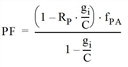
where

fPA	lookup value (HCM attachment 16 – 12) based on arrival type
RP	lookup value (HCM attachment 16 – 12) based on arrival type

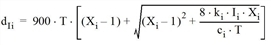
Step 10a: Calculation of the uniform delay for each lane group

The uniform delay is the delay expected given a uniform distribution for arrivals and no saturation. It is calculated as follows:

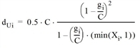
where

dUi	uniform delay for lane group i
gi	effective (actual) green time
Xi = v/c	volume/capacity ratio

Step 10b: Calculation of the incremental delay for each lane group

The incremental delay is the random delay that occurs since arrivals are not uniform and some cycles will overflow. It is calculated as follows:

where

dIi	incremental (random) delay for lane group i
ci	capacity for lane group i
Xi = v/c	volume/capacity ratio
T	duration of analysis period (hr) (default 0.25 for 15 min)
ki	lookup value (HCM attachment 16 – 13) based on the controller type
Ii	upstream filtering / metering adjustment factor (set to 1 for isolated intersection)

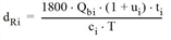
Step 10c: Delay calculation for the residual demand per lane group

Residual demand delay is the result of unmet demand at the beginning of an analysis period. It is only calculated if an initial unmet demand is entered for the beginning of the analysis period (Q). It is set to 0 in the current implementation. It is calculated as follows:

where

dRi	residual demand delay for lane group i
Qbi	initial unmet demand at the start of period T in vehicles for lane group (default 0)
ci	Capacity
T	Duration of analysis time slot (hr) (default 0.25 for 15 min)
ui	delay parameter for lane group (default 0)
ti	duration of unmet demand in T for lane group (default 0)

Step 11: Delay calculation for the approach

The total delay per vehicle for each lane group can be aggregated to the approach and to the entire intersection with the following equations. The approach delay is calculated as the weighted delay for each lane group.

where

dA	mean delay per vehicle for approach A
di	delay for lane group i
Vi	volume for lane group i

Step 12: Delay calculation for the intersection

The intersection delay is calculated as the weighted delay for each approach.

where

dI	mean delay per vehicle for intersection I
dA	delay for approach
VA	volume for approach

The HCM 6th Edition specifies how to define wait time for unsignalized movement, which can be taken into account for calculating the wait times for an approach or node. In this case, you need to list the values entered for calculation.

Step 13: Level of Service calculation

For the computation variant HCM 2000, the level of service is defined as a value which is based on the mean delay of the node.

LOS	Mean delay/vehicle
A	0 – 10 sec.
B	10 – 20 sec.
C	20 – 35 sec.
D	35 – 55 sec.
E	55 – 80 sec.
F	80 + sec.

In HCM 2010, the level of service is automatically classified as F if v/c (volume/capacity ratio) exceeds the value 1.

For the variants ICU 1, ICU2, and Circular 212, the level of service is defined through the saturation v/s (volume/saturation flow rate) of the node:

LOS	volume/saturation flow rate
A	0.000 - 0.600
B	0.601 - 0.700
C	0.701 - 0.800
D	0.801 - 0.900
E	0.901 - 1.000
F	>1.000

Step 14: Mean queue length calculation per lane group

Queue lengths are also calculated by the HCM 2000 method. In HCM 2010, the method differs. For this description, please refer to section 31-4, page 31-67 et seqq.

The equation for the calculation of the mean queue length is as follows:

Q = Q1 + Q2

where

Q	mean queue length – maximum distance measured in vehicles the queue extends on average signal cycle
Q1	mean queue length for uniform arrival with progression adjustment
Q2	incremental term associated with random arrival and overflow to next cycle

Step 14a: Calculation of the number of queued vehicles after the first cycle

Q1 represents the number of vehicles that arrive during the red stages and during the green stages until the queue has dissipated.

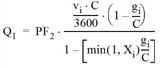
where

PF2	progression factor 2
vi	volume of lane group i per lane
C	cycle time
gi	effective green time of lane group i
Xi	volume/capacity ratio of lane group i

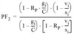
where

PF2	progression factor 2
vi	volume of lane group i per lane
C	cycle time
gi	effective green time of lane group i
si	saturation flow rate for lane group i
RP	platoon ratio – based on lookup table for arrival type

Step 14b: Calculate second-term of queued vehicles, estimate for mean overflow queue

where

T	Analysis period (usually 0.25 for 15 minutes)
k	adjustment factor for early arrival
Qb	initial queue at start of period (default 0)
ci	capacity for lane group i

k = 0.12 I • (sigi / 3,600) 0.7 for fixed-time signal

k = 0.10 I • (sigi / 3,600) 0.6 for demand-actuated signal

I	upstream filtering factor (set to 1 for isolated intersection)

Step 15: Calculation of the queue length percentile

After calculating the mean back of queue, the percentile of the back of queue is calculated as follows:

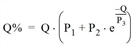
where

Q	Average queue length

percentile	pre-timed signal			actuated signal
	P1	P2	P3	P1	P2	P3
70%	1.2	0.1	5	1.1	0.1	40
85%	1.4	0.3	5	1.3	0.3	30
90%	1.5	0.5	5	1.4	0.4	20
95%	1.6	1.0	5	1.5	0.6	18
98%	1.7	1.5	5	1.7	1.0	13

Saturation flow rate adjustment factors

We now return to the calculation of the saturation flow rate (Saturation flow rate calculation by lane group), which involves several adjustment factors.

Step 6 a: Calculate lane width adjustment factor

where

fw	lane width adjustment factor
W	mean lane width (≥ 8) (ft)

This method differs in HCM 2010. For a description, please refer to HCM 2010, page 18-36.

Step 6b: Calculate heavy goods vehicle factor

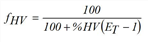
where

fHV	adjustment factor for heavy goods vehicles
%HV	percentage of HGV per lane group
EP	passenger car equivalent factor (2.0 / HV)

Step 6c: Calculate approach grade adjustment factor

where

fg	adjustment factor for approach grade
%G	approach grade as percentage (-6 % to +10 %)

In the HCM 6th Edition, the adjustment factors for heavy-goods vehicles and the slope of the approach were combined. The new, combined adjustment factors distinguish between negative slopes (gradients).

and non-negative slopes (level or pitch)

where

PHV	Share of HGV in lane group (%)
Pg	Slope of approach of lane group (%)

Step 6d: Calculate parking adjustment factor

fP is calculated as follows:

where

fp	parking adjustment factor (1.0 if no parking, otherwise ≥ 0.050)
N	number of lanes in lane group
Nm	number of parking maneuvers per hour (only for right turn lane groups) (0 to 180)

In Visum, enter fP which is calculated by the formula, as attribute ICA parking directly at the node leg.

Step 6e: Calculate adjustment factor for position to city center

fa = 0.9 if link is in the city center (CBD), otherwise 1.0

where

fa	adjustment factor for position
CBD	indicates a central business district

Step 6f: Calculate bus stop blocking factor

where

fbb	bus stop blocking adjustment factor (≥ 0.05)
N	number of lanes in lane group
NB	number of bus stop events per hour (does not apply to left turn lane groups) (0 to 250)

In Visum, enter fbb, the result obtained from the formula, as attribute ICA local bus stopping rate directly at the node leg.

Step 6g: Calculate lane utilization adjustment factor

where

fLu	adjustment factor lane utilization
vg	unadjusted (input) volume for lane group g
vgl	unadjusted (input) volume for lane with highest volume in lane group (veh per hour)

For this adjustment factor, an HCM lookup-table is regarded (HCM 2000: table 10-23 on page 10-26; HCM 2010: table 18-30 on page 18-77). Alternatively, lane attribute values can be used (ICA user-defined utilization share and ICA use user-defined utilization share).

Step 6h: Calculate right turn adjustment factor

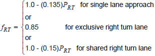
where

fRT	right turn adjustment factor (≥ 0.05)
PRT	proportion of right turn volume for lane group

The calculation according to HCM 2010 differs. For shared lanes, the adjustment factor is no longer explicitly calculated. For more details, please refer to HCM 2010, page 18-38.

Step 6i: Calculate left turn adjustment factor

The left turn adjustment factor is the most complex of the factors. Here, HCM 2000 and HCM 2010 differ significantly. For the description, please refer to HCM 2010, page 18-38 and pages 31-30 to 31-37. From the HCM 7th edition, the share of autonomous vehicles is taken into account in the calculation. The corresponding factors for secured and protected-plus-permitted left turns are found in Exhibits 31-65 and 31-66 of this issue.

The calculation is simple for protected left turns. However, if there is permitted phasing, then the equation is quite complex. It is as follows:

where

fLT	adjustment factor for left turns
PLT	proportion of left turn volume for lane group

For permitted staging, there are five cases. When there is protected-plus-permitted staging or permitted-plus-protected staging, the analysis is split into the protected portion and the permitted portion. The two are analyzed separately and then combined. Essentially this means treating them like separate lane groups. Refer to the HCM for how to split the effective green times among the protected and permitted portions.

1.  Exclusive lane with permitted phasing – use the general equation below

2.  Exclusive lane with protected-plus-permitted phasing – use 0.95 for the protected portion and the general equation below.

3.  Shared lane with permitted phasing – use the general equation below

4.  Shared lane with protected-plus-permitted phasing – use the equation above for protected phasing portion and the general equation below for the permitted portion

5.  Single lane approach with permitted left turns – use the general equation below

The general equation for calculating fLT for permitted left turns is listed below. Note that this is not the exact HCM 2000 equation since there are a few different versions depending on the situation – shared/exclusive lane, multilane/single lane approach, etc. But the equation is similar regardless of the situation. This general equation is the equation for an exclusive left turn lane with permitted phasing on a multilane approach opposed by a multilane approach.

The equation is basically the percentage of the time when lefts can make the turn times an adjustment factor. The adjustment factor is based on the portion of lefts in the lane group and an equivalent factor for gap acceptance time that is based on the opposing volume. The calculation of the percentage of the time when lefts can make the turn is a function of the opposing volume and their green time. The equation is as follows:

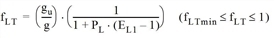
fLTmin = 2 • (1 + PL) / g

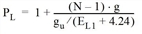
gu = g - gq (if gq ≥ 0, else gu = g)

where

fLT	Global adjustment factor for left-turns
fLTmin	Minimum value for adjustment factor
g	Effective non-protected green time for left-turn lane group
gu	Effective non-protected green time for left-turns crossing a conflicting flow
PL	Share of left-turns using lane L
EL1	Through equivalent for non-protected left-turns (veh/hr/lane) (look-up value depends on conflict flow volume)
gq	Effective non-protected green time, while left-turns are blocked completely and the spill-back of the conflict flow is reduced
go	Effective green time for conflict flow
N	Number of lanes in lane group
volc	Corrected conflict flow per lane per cycle =
No	Number of lanes in the lane group of the conflict flow
vo	Corrected conflict flow
fLUo	Lane utilization factor for conflict flow
qro	Opposing queue ratio = max[1 - Rpo • (go / C), 0] (Rpo = look-up value depends on ArrivalType)
tl	Loss time for left-turn lane group

The opposing volume is calculated from the signal groups that show green while the subject lane group has green. To calculate the opposing volume for a subject lane group, the entire opposing volume is used even if there is an overlap.

The permitted left movement calculation does not need to be generalized to 4+ legs since only one opposing approach is allowed. If more than one opposing approach is coded, an error is written to the log file.

Step 6j: Calculate pedestrian adjustment factors for left and right turns

Computation of the factors for left-turning and right-turning pedestrians and bicyclists is a considerably complex operation. It is performed in four steps. For the computation, the bicycle volumes of the legs are regarded and the pedestrian volumes of the crosswalks. A traffic flow has potential conflicts with two crosswalks on the outbound leg. These two crosswalks head for the opposite directions.

Note: At a leg which is a channelized turn no conflicts occur between right turn movements and pedestrians.

Step 1: Determination of the pedestrian occupancy rate OCCpedg.

The pedestrian occupancy rate OCCpedg is derived from the volume. The following applies:

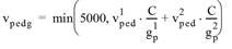
Here, vpedg is the pedestrian flow rate, v1pedg and v2pedg are the pedestrian volumes of the crosswalks, C is the cycle time of the signal control and g1p and g2p indicate the duration of the green for the pedestrians.

Note: In the HCM2000 it is implicitly assumed, that the green for the left turn movements and the green for the pedestrians start at the same time. In Visum, this is not the case, however. Thus, the following distinction of cases applies in Visum: If the pedestrian green time overlaps (or touches) the green or amber stage for vehicles, an existing conflict is assumed. In this case, the duration of the green of the pedestrian signal group is fully charged. Otherwise it is assumed, that there is no conflict. In this case, gp = 0 is assumed.

Step 2: Determination of the relevant occupancy rate of the conflict area OCCr

Here, three cases are distinguished:

• Case 1: Right turn movements without bicycle conflicts or left turn movements from one-way roads

In this case, the following applies:

OCCr = OCCpedg

Decisive for left turns from one-way roads is, that there is no opposing vehicle flow.

• Case 2: Right turn movements with bicycle conflicts

Here, straight turns of bicyclists are assumed.

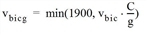
OCCbicg = 0.02 + vbicg / 2700

OCCr = OCCpedg + OCCbicg - (OCCpedg)•(OCCbicg)

Here, vbicg is the bicycle flow rate, vbic is the bicycle volume, C is the cycle time of the signal control, g is the effective green time of the lane group, and OCCbicg is the conflict area's occupancy rate caused by bicyclists.

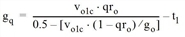
• Case 3: Other left turn movements

These are left turn movements which do not originate from a one-way road. Here, a distinction of cases is made for the values gq and gp. gq is the clearing time of the vehicle flow on the opposite leg, and gp is the green time for the conflicting pedestrians. The following applies:

gp = max(g1p, g2p)

• Case 3a: gq ≥ gp

In this case, the calculation is shortened and the following applies

fLpb = 1.0

Pedestrians and bicyclists are irrelevant here, since the left turn movements have to wait until the vehicle flow on the opposite leg is cleared.

• Case 3b: gq < gp

The following applies:

Here, OCCpedu is the occupancy rate of pedestrians after the clearance of the vehicle flow on the opposite leg, and OCCpedg is the pedestrians occupancy rate.

Step 3: Determination of the adjustment factors for pedestrians and bicyclists on permitted turns ApbT

Here, two cases are distinguished with regard to the values Nturn – which is the number of lanes per turn – and Nrec, which is the number of lanes per destination leg.

• Case 1: Nrec = Nturn

Here applies ApbT = 1 - OCCr

• Case 2: Nrec > Nturn

Here, vehicles have the chance to give way to pedestrians and bicyclists. The following applies:

ApbT = 1 - 0.6 • OCCr

Step 4: Determination of the adjustment factors for the saturation flow rates for pedestrians and bicyclists fLpb and fRpb.

fLpb is the adjustment factor for left turns, and fRpb is the adjustment factor for right turns. The following applies:

fRpb = 1 - PRT • (1 - ApbT) • (1 - PRTA)

fLpb = 1 - PLT • (1 - ApbT) • (1 - PLTA)

PRT and PLT represent the proportions of right turn and left turn movements in the lane group, and PRTA and PLTA code the permitted shares in the right and left turn movements (each referring to the total number of right turn and left turn movements of the lane group).

Step 6k: Calculating the adjustment factor for construction sites

The adjustment factor for the presence of construction sites is only applied from the 6th Edition of the HCM on. The latter takes the location of construction sites close to approaches to nodes into account. A construction site is considered close to an approach if it is 250 ft from its stop line or closer.

The adjustment factor can be calculated using the following equations:

≤ 1.0

with

where

fWZ	Adjustment factor for construction sites close to approaches
fwid	Adjustment factor for approach width
freduce	Adjustment factor for lane reduction due to construction site
aw	Lane width of approach during construction
no	Number of open left and straight lanes under normal conditions
nwz	Number of open left and straight extend during construction