Signal coordination (Signal offset optimization)

Signal cycle and split optimization always refer to individual signal controllers. Signal offset optimization, however, is used to optimize the offset between the signal times of neighboring nodes in such a way that vehicles can pass several consecutive signal controllers on green. The general aim is to minimize the total wait time for all vehicles signal controllers .

Notes: The method does not regard the attributes of the node geometry. In particular, the stop line position per lane is not taken into consideration. Signal coordination dos not include signalized nodes or main nodes to which no signal controller has been allocated or whose signal controller has been turned off.

Example

We will demonstrate the task with the help of the example network displayed in Image 286.

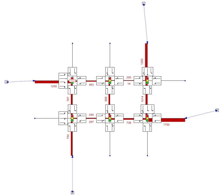
Image 286: Example network for signal coordination

In the network in Image 286, the six inner nodes have signal controls and the outer nodes are only there to connect the four zones. Link and turn volumes result from an assignment. Lane allocation is usually selected, so that at each approach of a node, a shared lane exists for the straight and right turns and a 100 m long pocket for left turns additionally. Additional lanes are only located at individual approaches with an especially large traffic volume. All signal controllers have the same signal times (Image 287).

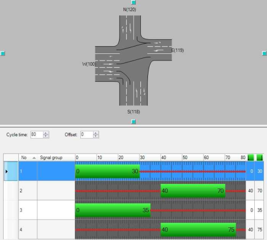
Image 287: Green time split at all nodes with succeeding left turns

With a cycle time of 80 s, straight and right turns each have a green time of 30 s. Signal groups for left turns have 5 s more and are protected within this time.

Signal times and lane allocation are selected in such a way that the resulting capacity is sufficient for all turns. Wait times can occur if neighboring signal controller are badly coordinated. For this example we first assume an offset time of 0 s for all signal controllers. The assignment result illustrated by link bars results as overlapping of seven paths and one of these is highlighted in Image 288.

Image 288: A path through the example network passes signal controllers at nodes 7003, 8003, 8002 and 9002

This route passes the signalized nodes 7,003, 8,003, and 9,002. Vehicles exiting node 7,003 in direction 8,003 form a group that starts at the beginning of the green time, i.e. at second 0. Travel time tCur, on the link between 7,003 and 8,003, is 38 s. Without accounting for dispersal of the group, the first vehicles reach node 8,003 at second 38. In fact, the distribution of the speeds actually traveled by the vehicles leads to a breakup of the originally compact platoon (Image 289).

Image 289: Progression quality for approach West at node 8003

On the left, the diagram shows the arrival rate by cycle second. The first vehicles arrive at second 30. The arrival rate then steeply increases and decreases as of second 52. The signal group to continue the journey also has a green time between second 0 and 30. The major part of the platoon therefore reaches the node at red. The second diagram shows the corresponding development of the queue length and the third diagram the resulting wait time in vehicle seconds dependant on the arrival second. The total wait time across all arrivals is 19,069 vehicle seconds, which corresponds to a mean value of 39.20 s per vehicle. This is an example for bad coordination.

At node 8002, the situation is much more favorable (Image 290).

Image 290: Progression quality for approach North at node 8002

The vehicle group again starts driving at second 0. The travel time on link 8,003 - 8,002, with tCur  = 41 s, is similar to before. However, the continuing signal group 4 for left turns, at node 8, has a green time from second 40 to second 75. Most of the vehicle group arrives during green time. The queues are distinctly shorter and the total wait time is only 1,608.80 vehicle seconds (mean: 4.37 s per vehicle).

In this simple example, the aim of signal coordination would be to change the offset between nodes 7,003 and 8,003, so that the entire vehicle group arrived at 8,003 during green time. At the same time, however, you would want to maintain the favorable offset between 8,003 and 8,0002. Because a convenient coordination should be achieved not only for one but several paths (in the example, seven) simultaneously, signal coordination usually minimizes the total wait time of all signal controllers by changing the offset times.

Model

Signal coordination in Visum can be used for optimizing signal controllers in a network, not only along a linear corridor, as it corresponds with the traditional optimization of the progressive signal system. This section describes how the optimization model is set up, which Visum solves by using a standard procedure for mixed integer linear optimization. All attributes that describe input and output of the procedure are summarized in the following section (Input attributes with effect at signal coordination).

Good coordination requires that the signal controllers either have the same cycle times or that the cycle times at least have a simple ratio (for example 2:1). Furthermore, signal controllers have to be located close to each other, otherwise the platoon will have broken up so heavily by the time it has reached the next signal controller, that the arrivals will virtually be uniformly distributed and the wait time cannot be influenced through the choice of the offset. It is therefore generally not sensible to coordinate all signal controllers in one network. You determine which signal controllers should be coordinated by defining signal coordination groups and assigning them signal controllers (User Manual: Managing signal coordination groups). By default, signal controllers are not assigned to any signal coordination group and are not coordinated.

For each signal coordination group define the set of the cycle times which are permitted for the corresponding signal controllers. Please make sure that the cycle times actually make coordination possible. Two signal controllers with cycle times of 60 s and 65 s can generally not be coordinated because the platoon in each cycle takes place at a different cycle second. Suitable cycle times therefore have a small LCM (least common multiple), for example, the family { 60 s, 80 s, 120 s } with LCM = 240 s. Signal coordination optimizes offset times for each signal coordination group separately and takes those signal controllers into consideration with cycle times belonging to the permitted cycle times of the group. Signal controllers with deviating cycle times are ignored and logged in the message file.

Important for coordination is the behavior of the vehicle platoon during the journey from one signal controller to another. Visum determines platoons by analyzing the assignment results for one or more selected PrT demand segments. From the saved paths of the assignment, Visum determines how many vehicles on their way first pass signal group SG1 of the signal controller SC1 and then signal group SG2 of the signal controller SC2. We call such a combination of two consecutive signal groups with one volume a coordination path leg or shorter path leg.

A path leg is relevant for the coordination if the following properties apply.

• The path leg starts and ends at signal controller of the same coordination group.
• The path leg contains no nodes (main nodes) of controller type All-way stop.
• The path leg passes through the node (main node) of controller type two-way stop only in the direction of the major flow.
• The path leg does not pass through other signalized nodes (main nodes).
• The travel time on the path leg is short enough so that a significant platoon is retained (specification below).
• No link along the path leg exceeds a threshold for the saturation.

All conditions except for the first one are aimed at a platoon to be retained along the path leg.

Optimization treats the traffic flows on all path legs independently. In each case it is assumed that within a cycle, all vehicles start as a platoon at the beginning of the green time. This means that beginning with the green time start, outgoing vehicles flow off with the saturation flow rate qmax, until the volume per cycle has been exhausted. The following applies:

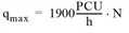
Here, N is the effective number of lanes for the turn. If the green time duration is insufficient and does not allow the volume allocated to a cycle from the assignment to exit with qmax, Visum ignores the excess volume and logs this in the message file.

The breakup of the platoon caused solely by different vehicle speeds is described by Robertson's platoon development formula. This model discretely divides the time in increments (in Visum of 1 s) and displays the number at time t‘, at which a vehicle arrives at the end of a path leg as a function of the number at time t < t‘, at the beginning of the path leg departing vehicle.

where

q‘t	the number of vehicles arriving at the end of the path leg in time step t
qt	the number of vehicles departing at the beginning of the path leg in time step t
F	with specified constants α and β
T	travel time tCur on the path leg

For the calculation of queue lengths, we assume idealistically that separate lanes of sufficient length exist for separate signal groups at an approach. Visum generally assumes "vertical" queues for signal coordination and does therefore not consider spillback upstream over several links or have an effect on the capacity of the turns of other signal groups.

For the evaluation of the progression quality, Visum calculates a number of skims which are used throughout literature. In the subsequent formulas CT determines the cycle time, GT the green time and qt the number of vehicles arriving at a node in time step t.

Platoon index = with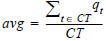

This size measures the "distance" of a volume profile of an equal distribution. The value varies from 0 (equal distribution) to 2 (for a distinct platoon). A high value means that coordination is worthwhile at this node, because the arriving vehicles are focused on part of the cycle time, so that there is a chance of moving the green time there, by changing the offset time.

Vehicles at green = .

This size directly measures how well coordination works. It calculates which part of the volume passes the node without stopping at the signal controller.

Platoon ratio =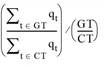

The size also measures how well coordination works, whereas high values imply good coordination. Especially high values are achieved when a large share of arrivals enter at green, although the green ratio itself is smaller.

The platoon ratio PR is the basis for the important ArrivalType parameter in waiting time calculations according to HCM.

ArrivalType =

Queue length queuet at a signal group to cycle second t results from the difference of cumulative inflows and exit flows. For this calculation, Visum also calculates the delays of travel times with specified arrival time in the queues and hence, the mean and total wait time.

Input attributes with effect at signal coordination

Signal coordination accesses the network objects and the input attributes displayed in Table 302.

Note: Node geometry attributes such as the stop line position, for example, are not regarded for signal coordination.

Network object	Attributes	Note
PrT paths	Volume	From assignment
Links, turns, main turns	Freely selectable attribute	Is interpreted as travel time and will be summed up for travel time calculation per path leg.
Signal controller with all components	All	Signal times and cycle time , mapping of signal groups and lane turns, selection of a reference signal controller that has an offset = 0.
Signal coordination groups	Cycle time family and assigned signal controller	Grouping of the signal controllers to be coordinated collectively

Table 302: Input attributes with an effect on signal coordination

Output attributes at signal coordination

The effect of the signal coordination is primarily to assign the optimal value to the offset attribute of the coordinated signal controller.

Alongside that, all skims listed above can be calculated for measuring the progression quality. Their definitions first of all refer to a single path leg. In order to easier display results in a network model, Visum aggregates the values of all skims on links and saves the results as link attributes. Visum allocates the attributes at all approach links to signalized nodes which have a volume of > 0. All link attributes for signal coordination results are contained in Table 303.

Table 303: Output attributes of links for results of signal coordination

Name	Value type	Value range	Meaning
Signal controller coordination vehicles on green	Double	0.0 .. 100.0	Number of vehicles which arrive during green time [%]
SC coord platoon index	Double	0.0 .. 2.0	Definition see above
SC coord platoon ratio	Double	0.0 ..	Definition see above
SC coord arrival type	Integer	1 .. 6	Definition see above
SC coord wait time	Time	0 s ..	Total wait time [Vehicle seconds] Note: For links to overloaded signal groups, this value is set to 100,000 h.
SC coord maximum queue length	Double	0.0 ..	Max. number of queued vehicles over all cycle seconds [Veh] Note: For links to overloaded signal groups, this value is set to 100,000.

Note: By the name component 'SC coord', the attribute SC coord arrival type is indicated as signal coordination output attribute. It is not identical to the ICA arrival type attribute, which is used as entry for ICA calculation. If you want to calculate the ICA impedance with an arrival type which corresponds with the given offset time intervals, first perform the Signal offset analysis and then copy the SC coord arrival type values to the ICA arrival type attribute.

Procedure parameters

Besides the network object attributes, the procedure parameters listed in Table 304 control signal coordination.

Name	Value range (Standard)	Meaning
Automatic Analysis	Boole (True)	After signal coordination, the output link attributes are automatically updated.
Coordination group set	Set of coordination groups (all)	Coordination is only carried out optionally for selected signal coordination groups.
Demand segments set	Set of assigned PrT_DSeg (all assigned PrT_DSeg)	Optionally, path legs are only determined from the assignment paths of selected demand segments.
MaxSaturation	Double > 0 (80%), in percent	If this saturation is exceeded on a path leg link, the path leg is ignored for coordination, because no platoon is retained with too high saturation.
MinPlatoonIndex	Double > 0 (0.4)	If the platoon index is below this threshold at the end of the path leg, the path leg is ignored for coordination, because the platoon is not distinct enough.
RobertsonAlpha	Double > 0 (0.35)	Parameter for the platoon progression formula according to Robertson
RobertsonBeta	Double > 0 (0.8)	Parameter for the platoon progression formula according to Robertson
TravelTimeLinkAttr	numeric link attribute (AddValue1)	When calculating the path leg travel time, for each traversed link, TravelTimeLinkFac • TravelTimeLinkAttr is summed up
TravelTimeLinkFac	Double > 0 (1.0)
TravelTimeTurnAttr	Numeric turn attribute (AddVal1)	When calculating the path leg run time, for each traversed turn, TravelTimeTurnFac • TravelTimeTurnAttr is summed up
TravelTimeTurnFac	Double > 0 (1.0)
TravelTimeMainTurnAttr	Numeric main turn attributes (AddVal1)	When calculating the path leg run time, for each traversed turn, TravelTimeMainTurnFac • TravelTimeMainTurnAttr is summed up
TravelTimeMainTurnFac	Double > 0 (1.0)
MaxCalculationTime	Time	Calculation time for the solution of the optimization problem is restricted. The best solution found up to the specified time limitation, is assigned.

Table 304: Procedure parameters for signal coordination

Problem solution

To determine an optimal set of offset times per signal controller, Visum sets up a mixed integer linear optimization problem. The deciding variables in this problem are the differences of the offset times of neighboring signal controllers, the objective function is an in sections linearized approximation of the wait time in dependency thereof. Secondary conditions express that the differences between the offset times of adjacent signal controllers along each circle in the network have to be added to an integer multiple of the cycle time.

A detailed description of the method is found in Möhring, Nökel, Wünsch 2006.