|
Note: For the description of this control type, please refer to HCM 2000, chapter 17 (in HCM 2010, refer to chapter 20 and in HCM 6, to chapter 21). The calculations described in HCM 2010 and HCM 2000 are identical. HCM 2010 additionally includes the guidelines for queue length calculations (HCM 2010, page 20-17), which is missing in HCM 2000. Furthermore, the volume/capacity ratio is regarded for the LOS calculation. In the event of a capacity overload, the LOS is automatically F. The calculation in HCM 6 |
The HCM 2000 all-way stop controlled (AWSC) capacity analysis method is an iterative method. The model looks at all possible scenarios of a vehicle either being at an approach or not being at an approach. Based on the input volumes the probability of each scenario occurring is calculated as well as the mean delay. The v/c ratio is calculated for each scenario which in turn impacts the others. Therefore, an iterative solution is needed to find the capacity of each approach.
Unlike the signalized method, which works with signal groups, or the TWSC method, which works with movements, the AWSC model works with lanes by approach.
The basic calculation is described in the flow chart in Image 76. The user inputs intersection geometry and volumes, along with a couple of additional attributes such as PHF and %HGV. The volumes are adjusted and allocated to the lanes. The next step is to calculate the saturation (capacity) follow-up time adjustment factors. Then the departure follow-up times (i.e. the mean time between departures for a lane at an approach) are calculated based on all the combinations of the probability states. This departure follow-up time for each lane for each approach is dependent on the other approaches and so it is calculated in an iterative manner. Once a converged value is found, then the service time, mean delay and LOS can be calculated.

Image 76: Calculation process for an all-way stop node
If you use the HCM operations model for all-way stop nodes, the following Visum attributes, listed in Table 109, will show an effect. Make sure that they are set to realistic values prior to running the analysis.
|
Network object |
Attribute |
Description / Effect |
|
Node |
ICAPHFVolAdj |
Initial volume adjustment to peak period. Then, volumes are divided by both node and turn adjustment factors. |
|
Geometry |
All |
Geometry information on lanes, lane turns and crosswalks |
|
Turns |
ShareHGV |
Proportion of heavy goods vehicles, used in follow-up times adjustment. Fixed value that applies for turns. |
|
Turn |
ICAPHFVolAdj |
Initial volume adjustment to peak period. Then, volumes are divided by both node and turn adjustment factors. |
| Turn | ICA average back of queue | Average queue length |
Output is available through the same attributes as for signalized nodes (Table 100).
The first step is to PHF adjust the volumes by lane by movement by approach. In addition the % heavy goods vehicles by lane by movement by approach are also input if available. Since in Visum volumes are specified by movement and not by lane by movement, they are first disaggregated per lane according to a standard method.
The next step is to calculate the follow-up time adjustment factors for each lane. The calculation applies as follows:
hadj = hLTadj • pLT + hRTadj • pRT + hHVadj • pHV
where
|
hadj |
follow-up time adjustment |
|
hLTadj |
follow-up time adjustment for left turns |
|
hRTadj |
follow-up time adjustment for right turns |
|
hHVadj |
follow-up time adjustment for heavy vehicles |
|
PLT |
proportion of left-turning vehicles on approach |
|
pRT |
proportion of right-turning vehicles on approach |
|
pHV |
proportion of heavy vehicles on approach |
The adjustment factors are listed in Table 110.
|
Number of lanes of the subject approach |
Adjustment factor |
Saturation |
Follow-up time |
|
|
LT |
RT |
HV |
|
1 |
0.2 |
-0.6 |
1.7 |
|
2+ |
0.5 |
-0.7 |
1.7 |
After calculating the follow-up time adjustment factor the departure follow-up time is calculated in an iterative manner. It involves five steps.
Step 1: Calculate combined probability states probability

where
|
P(i) |
probability for combination i |
|
P(aj) |
probability of degree-of-conflict (DOC) for combination i lane type j |
|
aj |
1 or 0, depending on lane type j (see Table 111) |
This probability states calculation has a few parts. For each lane type j the P(aj) is calculated. P(aj) is calculated based on a lookup table (Table 111).
|
aj |
Vj (volume conflicting approach) |
P(aj) |
|
1 |
0 |
0 |
|
0 |
0 |
1 |
|
1 |
>0 |
Xj |
|
0 |
>0 |
1 - Xj |
|
Notes:
|
Value aj is adopted from the DOC table (Table 112). This table contains all the combinations of 0 and 1 per lane for each approach. For two lanes per approach, this looks as depicted in Table 112 (see exhibit 17-30 in the HCM 2000 for the full table).
|
i |
DOC case (Ck) |
Number of vehicles |
Opposing approach |
Left (subject approach) |
Right (subject approach) |
|||
|
|
|
|
L1 |
L2 |
L1 |
L2 |
L1 |
L2 |
|
1 |
1 |
0 |
0 |
0 |
0 |
0 |
0 |
0 |
|
2 |
2 |
1 |
1 |
0 |
0 |
0 |
0 |
0 |
|
3 |
2 |
1 |
0 |
1 |
0 |
0 |
0 |
0 |
|
4 |
2 |
2 |
1 |
1 |
0 |
0 |
0 |
0 |
|
… |
|
|
|
|
|
|
|
|
|
64 |
There are 64 combinations for 4 legs each with 2 lanes. |
|||||||
The combined probability states probability P(i) is then calculated for each row (i) for each column (lane type) (j). To calculate P(i), we use the product of all probabilities of each opposing lane and each conflicting lane P(aj) . The result P(i) = ∏P(aj) is the probability state for row (i).
Step 2: Calculate probability state adjustment factors
After calculating P(i) for each case (i), an adjustment for each DOC case needs to be calculated. The adjustment accounts for serial correlation in the previous calculation due to related conflict cases. For DOC case (Ck), the adjustment equations are:

where
|
a |
0.01 (or 0.00 if no serial correlation) |
|
n |
number of non-zero cases (i) for each DOC case (at most n = 1 for C1, 3 for C2, 6 for C3, 27 for C4 and C5) |
Step 3: Calculate adjusted probability
P‘(i) = P(i) + adjP(i)
where
|
P‘(i) |
adjusted probability for case i |
|
P(i) |
probability of degree-of-conflicts for case i |
|
adjP(i) |
probability adjustment factor case i |
Step 4: Calculate saturation follow-up time
hsi = hadj + hbase
where
|
hsi |
saturation follow-up time by DOC case i |
|
hadj |
follow-up time adjustment by lane |
|
hbase |
base follow-up time by DOC case i |
For each DOC case i, the base follow-up time hbase is adopted from a lookup table which is based on the particular DOC case (1 – 5) and geometry group (Table 113).
|
Number of lanes |
||||
|
Subject approach |
Opposing approach |
Unpermitted approach |
Intersection type |
Geometry group |
|
1 |
1 |
1 |
4 leg or T |
1 |
|
1 |
1 |
2 |
4 leg or T |
2 |
|
1 |
2 |
1 |
4 leg or T |
3a / 4a |
|
1 |
2 |
2 |
T |
3b |
|
1 |
2 |
2 |
4 leg |
4b |
|
2 |
1 - 2 |
1 - 2 |
4 leg or T |
5 |
|
3 |
1* |
1* |
4 leg or T |
5 |
|
3 |
3 |
3 |
4 leg or T |
6 |
|
Note: * If the approach examined has 3 lanes and the opposing or conflicting approach has 1 lane, then geometry group 5 applies, else geometry group 6. |
The model is generalized for 3+ lanes in order to apply it to 4+ leg intersections. The extension is that these 4+ leg cases are geometry group 6.
The Table 114 shows the saturation follow-up time base values.
|
DOC case |
1 |
2 |
3 |
4 |
5 |
|
|
|
Number of vehicles (Sum of the [0,1] for the case) |
0 |
1 2 >=3 |
1 2 >=3 |
2 3 4 >=5 |
3 4 5 >=6 |
|
Geometry group |
1 |
3.9 |
4.7 |
5.8 |
7.0 |
9.6 |
|
2 |
3.9 |
4.7 |
5.8 |
7.0 |
9.6 |
|
|
3a |
4.0 |
4.8 |
5.9 |
7.1 |
9.7 |
|
|
3b |
4.3 |
5.1 |
6.2 |
7.4 |
10.0 |
|
|
4a |
4.0 |
4.8 |
5.9 |
7.1 |
9.7 |
|
|
4b |
4.5 |
5.3 |
6.4 |
7.6 |
10.2 |
|
|
5 |
4.5 |
5.0 6.2 |
6.4 7.2 |
7.6 7.8 9.0 |
9.7 9.7 10.0 11.5 |
|
|
6 |
4.5 |
6.0 6.8 7.4 |
6.6 7.3 7.8 |
8.1 8.7 9.6 12.3 |
10.0 11.1 11.4 13.3 |
|
The DOC case is dependent on the 64 types of a 4 leg intersection. Nodes with more than 4 legs are first collapsed to four legs.
Step 5: Calculate departure follow-up time

where
|
hd |
departure follow-up time for lane |
|
hsi |
saturation follow-up time for each i in I |
|
P‘(i) |
adjusted probability for each i in I |
|
I |
Row of Table 109 |
These five steps are repeated until the departure follow-up time values converge (change is < 0.1). Now, the calculated departure follow-up time hd differs from the original value. Thus, the next iteration will return a different result.
Now that the departure follow-up time for each lane is calculated, service time and capacity can be calculated. The service time is calculated as follows:
t = hd - m
where
|
t |
Service time |
|
hd |
Departure follow-up time |
|
m |
move up time (2.0 s for geometry groups 1-4 and 2.3 s for groups 5-6) |
The capacity is calculated as follows: the volume of the subject lane is incremented until its degree of utilization (vjhd)/ 3,600 is ≥ 1.0. The volume of the other approaches is held constant. At this point, the subject lane’s volume value is taken to be the subject lane’s capacity. Capacity is therefore dependent on the input volumes for each approach.
The search for capacity is slow in a linear implementation. Thus a binary search is performed with an upper bound of 1,800 vphpl.
Mean delay per lane is calculated from the equation below. The weighted mean delay for an approach is calculated based on lane volume weights. Intersection average delay is calculated based on the weighted mean by approach volumes. The equations are the same as the ones for signalized intersections.
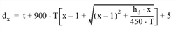
where
|
dx |
Mean delay per vehicle for lane x |
|
t |
Service time |
|
T |
Duration of analysis time slot (hr) (default 0.25 for 15 min) |
|
x |
Utility rate |
|
hd |
Departure follow-up time |

Level of Service is defined as a lookup, based on intersection delay (Table 115).
|
LOS |
Mean delay/vehicle |
|
A |
0 – 10 s |
|
B |
10 – 15 s |
|
C |
15 – 25 s |
|
D |
25 – 35 s |
|
E |
35 – 50 s |
|
F |
50 + s |
The proposed extension to 4+ legs is to combine multiple lefts or rights into one left or right by adding the number of lanes when calculating conflicting flows. For example, when there are two conflicting lefts for an examined approach, one with one lane and one with two lanes, these are merged into one conflicting left with three lanes. This allows the existing framework to be used. It probably slightly understates the delay, but it will work within the existing framework and will result in additional delay for additional legs.
