In case of an hypercritical or hypocritical speed measure (please see → Link model), you can adopt different policies to correct the speed measures.
Currently, you can use two different algorithms.
- Fundamental Diagram Correction (FDC).
- Queue Correction (QC).
According to the configuration of the TRE parameter HypercriticalSpeedMeasureSetQueue (see → Traffic data parameters) you can use:
- Both FDC and QC for hypocritical speed measures corrections.
- QC for hypecritical speed measures corrections.
The effects of a speed measure vm are modeled by a modification of the fundamental diagram of the link that is affected by the measure.
Given the flow level qc currently crossing the entry section, the fundamental diagram parameters V and Q (and as a subsequence Φ and K) are modified so that v°(qc) = vm.
As the problem has infinite solutions (one parabola per two points), we additionally impose the following arbitrary condition:
Q’ / V’ = Q / V
This means that the ratio between the nominal capacity and the free flow speed is conserved (they are increased or decreased proportionally).
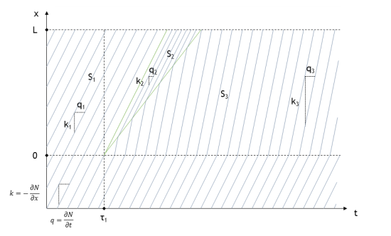
Image 1 and image 3 below show the switched fundamental diagrams and the origin, destination, and transition states for cases of speed decrease and increase. Image 2 and image 4 show the vehicle trajectories on a common space-time diagram for cases of speed decrease and increase.
Important: Note that the theoretical General Link Transmission Model (GLTM) only controls entry and exit sections of links. During the measure’s validity, the modification can only affect the new vehicles entering the link but not the vehicles already traveling along the link. This means that the speed of vehicles that passed the entry section before the event is not affected and subsequently they could slow down or separate respectively faster or slower trailing vehicles.
Image 1: Fundamental diagram switch in case of decreasing free flow speed
The new fundamental diagram (FD2) parameters are computed in order to obtain a flow speed equal to the measured flow speed when the flow value is the same as the value in the state S1.
The transition state S2 is the state on the new fundamental diagram with a flow speed equal to the speed in S1. If the speed in S1 is greater than the free flow speed of the new fundamental diagram (see the left panel in image of the example below), the transition state S2 will result in a null flow.
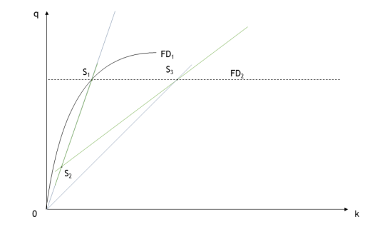
Image 2: Vehicle trajectories in case of decreasing free-flow speed
The state S1, corresponding to the state before the measure, is propagated through the link after the measure until the arrival time of the shock wave S1−S2. Then the transition state S2 is propagated up to the arrival time of the shock wave S2−S3. Finally, the new fundamental diagram affects the flow propagation on the link.
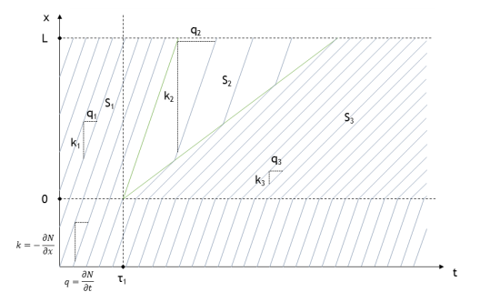
Image 3: Fundamental diagram switch in case of increasing free-flow speed
Contrary to the previous case (image 1), if the new fundamental diagram has a greater free flow speed than the original fundamental diagram, the flow value corresponding to the transition state S2 will be greater than the original flow. Anyway it is bounded by the new link capacity.
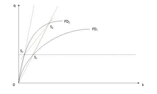
Image 4: Vehicle trajectories in case of increasing free flow speed
As in image 2, the two shock waves S1−S2 and S2−S3 are computed and the three states are propagated accordingly along with the shock wave arrival times.
The next image shows a speed measure effect on the fundamental diagram of a link (a) and the resulting cumulative exit flow correction (b).
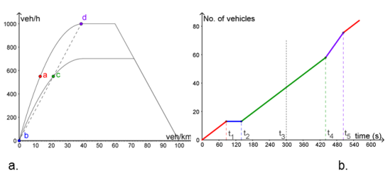
In the example, a speed of 25 km/h is measured on a link with a free flow speed of 50 km/h and a length of 1 km. The measure applies from time 0 s to 300 s. A constant flow of 550 veh/h enters the link. Immediately before the measure, the vehicles were traveling in a flow state with a speed of ~42 km/h (point a in a.). The measure then slows down the link traffic conditions (standard behavior as from the original fundamental diagram), switching from the greater fundamental diagram to the smaller one. The new fundamental diagram parameters are tuned so that the flow speed corresponding to the flow value experimented at the start of the measure is equal to the measured speed. Points a, b, c, d show the different states that the traffic goes through. We call b and d the transition states.
A transition state is determined as the state on the new fundamental diagram that has the same speed as the previous state on the previous fundamental diagram. Of course, it is constrained to provide a speed not greater than the new free flow speed V’, nor a capacity greater than the new physical capacity Q’.
Example: In this example, the traffic state speed of a is ~42 km/h. This is greater than the new fundamental diagram free flow speed of 35 km/h. The resulting transition state b has a speed of 35 km/h and a flow of 0 veh/h.
Because the vehicles already on the link are not affected by the speed correction, the effect of the measure on the exit flow is delayed until time t1. The vehicles will reach the head of the link at their original speed. This means that the flow state a is propagated until the shock wave between states a and b reaches the link head (red segment in the image).
Vehicles that enter the link during the measure validity at the flow level of the original state a will travel exactly at the measured speed. As a subsequence, the shock wave started at t0 = 0 will reach the head of the link at t2. In the example, as the transition state b is 0 veh/h, the speed of the shock wave between the states b and c also coincides with the vehicle speed of 25 km/h, and [t0,t2] is also the vehicle travel time. For the same reason, in this example no vehicle will leave the link in the interval [t1,t2] (flat blue segment of the cumulative flow plot). This is because the slower newly entering vehicles were distanced by the faster previous vehicles.
From instant t2, the new fundamental diagram states also apply to the exit flows because the state c has reached the head of the link.
At time t3, the measure validity ends and the original fundamental diagram is restored. However, the shock wave between the states c and d will reach the head only at time t4. During the interval [t4,t5], the exit flow is in a transition state at the point d of the original fundamental diagram, determined as the state with a speed equal to the speed of c. This transition state holds until the instant t5, which is the arrival time of the shock wave between the states d and a.
Note that in case of a speed measure faster than the original free flow speed of the link, the cycle a–b–c–d–a would have been c–d–a–b–c with the same logic.
In this model possible inconsistencies can occur during the simulations for the effect of a delay at the link head results in an increased travel time (see → Signals).
The travel time has a lower bound set by the delay amount. Accordingly, the maximum free flow speed is equal to the ratio between its length and such a delay.
The theoretical model does not allow waves and thus does not allow vehicles to propagate slower than defined by the parameter MinWaveSpeed (see → Supply parameters) that is the minimum free flow speed.
In case the measured speed is out of these bounds, it cannot be reproduced in the simulation.
In case a hypercritical speed measure is received, you can have two effects:
- The FD hypocritical branch is modified so that the travel time along the link coincides with the one at the measured speed.
-
The link exit capacity bottleneck is set to the flow value at the intersection between the FD hypercritical branch and the speed secant.
The combination of the two effects, plus any possible more severe bottleneck as spillback from downstream, can imply a limitation for the traffic flow.
If any of the downstream bottlenecks limits the flow once it has travelled the wished travel time, there is:
- An additional queue delay.
- The travel time is higher than the measured one
- The speed is lower on the upstream link.
Hypercritical speed correction
The speed is computed as the average between hypocritical and hypercritical speed weighted by the number of vehicles in hypocritical and hypercritical state.
The goal is to match the measured and result speed values:
Vresults = Vhypo•(1-quen)+Vhype•(quen) = Vmeasures (1)
Where:
Vhypo = Q0(k0)/(k0)
Vhype = Q+(k+)/(k+)
k0 = (nveh•(1-quen))/(L•(1-quel))
k+ = (nveh•quen)/(L•quel)
Replacing in the relation (1) the previous four definitions, you get:
Vresults = Q0(k0•(L•(1-quel)/nveh)+Q+(k+)•(L•quel/nveh) = Vmeasures (2)
Where:
quel = queu/(queu+stor)
nveh = F-E+D
stor = Gt -F+D
queu = Ht -E+D
If flows are constant, we have:
Q0(k0) = Qt0 (3)
Q+(k+) = Qt+ (4)
If flows are not constant, for a generic fundamental diagram we have:
Q0(k0) = Q•[1 - (1 - (k0•V)/(Q•γ0))^γ0] (5)
Q+(k+) = Q•[1 - (1 + ((k++J)•W)/(Q•γ+))^γ+] (6)
In case of constant flows, we can easily solve the equation (2) with respect to D:
D = [(F-E)•V•L-Qt0+ (Ht - E)•((Qt+-Qt0)/(Ht - E + Gt -F))]/[(Qt+-Qt0)/(Ht - E + Gt -F)-V•L] (7)
If the flows are not constant, the explicit solution of equation (2), substituting Q0 and Q+ with equations (5) and (6), is harder, and a simple iterative algorithm is used instead.