Link model

The traffic along the link a is represented in the space x and the time τ as a macroscopic, unidimensional fluid of partially compressible particles.

We introduce five main variables (we omit the index a for simplicity of notation):

• N(x,τ) is the total number of vehicles that traversed section x until time τ
• q(x,τ) = ∂N(x,τ) / ∂τ   flow through section x at time τ
• k(x,τ) = -∂N(x,τ) / ∂x   density at section x and time τ
• v(x,τ) = q(x,τ) / k(x,τ)   flow speed at section x and time τ, where dN(x,τ) = 0
• w(x,τ) = dq(x,τ) / dk(x,τ)   wave speed at section x and time τ where dq(x,τ) = 0

The fundamental diagram q = q(k) shown in the next image is the experimental relation between flow and density:

 

 

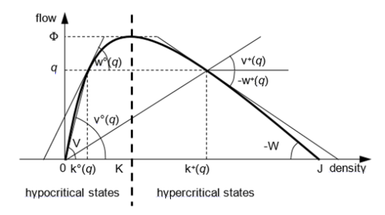
The fundamental diagram represents the two main phenomena of driver behavior when driving along a road channel that has homogeneous characteristics and no bottlenecks. These main phenomena are:

• The variance of the desired speed in free flow conditions among different vehicles, assuming no overtaking so that the frequency of delays due to a slower car ahead increases with the density of the flow (hypocritical spacing)
• The need for a vehicle to keep a safety distance to the car ahead, which depends on the speed of the flow (hypercritical spacing)

The fundamental diagram holds for stationary conditions.

Kinematic Wave Theory is valid also for non-stationary traffic flows. This implies that vehicles react instantaneously to changing flow states with no reaction time (although their spacing takes it into account) by adapting their speed without instabilities.

Referring separately to the two branches (hypocritical and hypercritical) of the fundamental diagram, we can then introduce the following functions of the flow:

k°(q) = q-1(q)	hypocritical density (trivially k°(0) = 0)	(1)
v°(q) = q / k°(q)	hypocritical vehicle speed	(2)
w°(q) = 1 / [dk°(q) /dq]	hypocritical wave speed	(3)
k+(q) = q-1(q)	hypercritical density	(4)
v+(q) = q / k+(q)	hypercritical vehicle speed	(5)
w+(q) = 1 / [dk+(q) /dq]	hypercritical wave speed	(6)

All the parameters defining the shape of one branch of the fundamental diagram are assumed to be constant in space and time. We denote in particular:

V = v°(0) = w°(0)	free flow speed	(7)
W = -w+(0)	jam wave speed	(8)
J = k+(0)	jam density	(9)
ɸ = max{q(k): k∊[0, J]}	physical capacity	(10)
Q = UB{q(k)}	nominal capacity	(11)
K = k°(ɸ) = k+(ɸ)	critical density	(12)
γ°	hypocritical curvature	(13)
γ+	hypercritical curvature	(14)

Classical forms of the fundamental diagram are:

• The triangular form
• The parabolic form

The parameters “free flow speed” (7) and “hypercritical curvature” (14) are rather physical quantities. They can be robustly estimated by direct measurements although we often recur to model transposition and previous experience.

We introduce both a physical capacity F and a nominal capacity Q because sometimes the input capacity of the model (Q) is neglected if unrealistic (see image of fundamental diagram).

There is some degree of correlation among these parameters, but they can be considered independent of each other.

In practice, there are road types with all sorts of value combinations. Several mathematical models were proposed by researchers for fundamental diagrams: among these are Newell (1993), Greenshield (1935), Greenberg (1959), Underwood (1961), and Del Castillo (2011).

The fundamental diagram form used in TRE is the Gentile polynomial model.

It defines the fundamental diagram as two distinct branches, with the following equations:

q°(k) = Q•(1-(1-(k•V)/Q•γ°)^γ°)	k <= γ°•(Q/V)	(15)
q°(k) = Q	otherwise
q+(k) = Q•(1-(1+((k-J)•W)/Q•γ+)^γ+)	k >= J-γ+•(Q/W)	(16)
q+(k) = Q	otherwise

The model can thus formally be described as:

q(k) = min{q°(k), q+(k), Q}   (17)

From (15)−(16) we can write (1)−(6) for q∊[0, Q] as follows:

k°(q) = γ° • Q / V × [1 - (1- q / Q)1/γ°]  (18)

k+(q) = J - γ+ • Q / W • [1 - (1- q / Q)1/γ+]   (19)

w°(q) = V • (1 - q / Q)1-1/γ°   (20)

w+(q) = -W • (1 - q / Q)1-1/γ+   (21)

v(q) = q / k(q)   (22)

dv(q)/dq = [1 - v(q) / w(q)] / k(q)   (23)

Note that because the two branches have independent formulas, the actual model capacity Φ of the link may be lower than the input capacity Q, depending on the shape parameters of the two branches. The physical capacity is defined as:

Φ = max{q(k): k∊[0, J]}   (24)

Example:

The next image shows the actual link maximum flow.

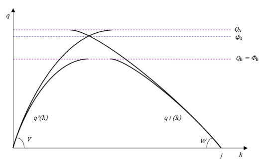
Q_A is a flow state actually unachievable. Despite the shapes of the two branches, it yields to a maximum flow of Φ_A, smaller than Q_A.

On the contrary, Q_B is a feasible flow value and the resulting physical capacity Φ_B coincides with Q_B. Also, in this case for a range of density states the resulting flow is identically Q_B (flat shape in the range between the two branches).

This model is responsible for updating the potential sending flow of future instants at the exit of the link according to the current and previous flow states at the entrance of the link.

Given a link length L > 0, let f(τ) = q(0,τ) be the link inflow at time τ (x = 0 is the initial section). By definition, the cumulative inflow, that is the number of vehicles that passed the initial point of the link until τ, is given by:

F(τ) = N(0,τ) = ₀⎰^τf(ζ) • dζ   (25)

The instant u(x,τ) ≥ τ when the forward kinematic wave generated at time τ on the initial point of the link by the hypocritical inflow f(τ) reaches section x, is given by:

u(x,τ) = τ + x / w°(f(τ))   (26)

In general, u(x,τ) is not invertible because more than one kinematic wave generated on the initial point may reach the final point at the same time (for decreasing inflows). If f(τ) is the prevailing flow state at time u(x,τ) in the final point, the corresponding cumulative flow Ĥ(x,τ) is given by F(τ) plus the number of vehicles that have passed the forward kinematic wave with slope w°(f(τ)) generated at τ in the initial point:

Ĥ(x,τ) = F(τ) + f(τ) • x • [1 / w°(f(τ)) - 1 / v°(f(τ))]   (27)

The next image shows a space-time diagram of a forward kinematic wave and traversing vehicle trajectories:

The Newell-Luke Minimum Principle (NLMP) states that among all forward kinematic waves that reach the final point at time τ, the one yielding the minimum cumulative flow dominates the others. This kinematic wave is denoted H(τ).

H(x,τ) = min{Ĥ(x,σ): u(x,σ)= τ}   (28)

According to this, when u(x,τ) will be the current instant, the prevailing state and thus the current sending flow will be known.

This model is responsible for updating the potential receiving flow of future instants at the entrance of the link according to the current and previous flow states at the exit of the link.

Given a link length L > 0, let e(τ) = q(L,τ) be its outflow (x = L is the final section of the link at time τ). By definition, the cumulative outflow, that is the number of vehicles that passed the final point of the link until the instant, is given by:

E(τ) = N(L,τ) = ₀⎰^τe(ζ) • dζ   (29)

The instant z(x,τ) ≥ τ when the backward kinematic wave generated at time τ on the final point of the link by the hypercritical outflow e(τ) reaches the initial point, is given by:

z(x,τ) = τ - L / w+(e(τ))   (30)

Similar to the hypocritical wave forward propagation model, z(x,τ) is not invertible because more than one kinematic wave generated on the final point may reach the initial point at the same time (for decreasing outflows). If e(τ) is the prevailing flow state at time z(x,τ) in the initial point, the corresponding cumulative flow Ĝ(x,τ) is given by E(τ) plus the number of vehicles that have passed the backward forward kinematic wave with (negative) slope w+(e(τ)) generated at τ in the final point:

Ĝ(x,τ) = E(τ) + e(τ) • x • [-1 / w+(e(τ)) + 1 / v+(e(τ))]   (31)

The next image shows a space-time diagram of a backward kinematic wave and traversing vehicle trajectories:

The Newell-Luke Minimum Principle (NLMP) states that among all backward kinematic waves that reach the initial point at time τ, the one yielding the minimum cumulative flow dominates the others. This backward kinematic wave is denoted G(τ).

G(x,τ) = min{Ĝ(ζ): z(ζ) = τ}   (32)

According to this, when z(x,τ) will be the current instant, the prevailing state and thus the current receiving flow will be known.

The exit capacity of the link is specified by its attribute ocap.

Important:  The link exit capacity can be modified by the modifications to the fundamental diagram (→ Link model).

Link model attributes can be temporarily modified by temporary attributes.

The following temporary attributes can affect the simulation:

Attribute	Description
CAPA	Affects the capacity of a link, both entry and trunk (then fundamental diagram). The exit capacity of the link is not affected. This means that if a queue is present on the link, it continues dispersion at the same exit rate.