Visum provides several assignment procedures for the PrT. There are static assignment procedures without explicit time modeling as well as procedures that use a time dynamic traffic flow model.
- The Incremental assignment divides the demand matrix on a percentage basis into several partial matrices. These partial matrices are then successively assigned to the network. The route search accounts for impedance resulting from the traffic volume of the previous step (Incremental assignment).
- Equilibrium assignment distributes the demand according to Wardrop's first principle: "Every road user selects his route in such a way that the travel time on all alternative routes is the same, and that switching to a different route would increase personal travel time.”
- The Equilibrium assignment LUCE uses the LUCE algorithm, which was conceived by Guido Gentile. He collaborated with PTV to produce a practical implementation of the method in Visum. Exploiting the inexpensive information provided by the derivatives of the arc costs with respect to arc flows, LUCE achieves a very high convergence speed, while it assigns the demand flow of each OD pair on several paths at once (Linear User Cost Equilibrium (LUCE)).
- The Equilibrium assignment Bi-conjugate Frank Wolfe is a further development of the method Frank Wolfe (FW). The assignment procedure was implemented based on the publication of Mitradjieva, Lindberg et al (2013) (Bi-conjugate Frank-Wolfe (BFW)).
- The Equilibrium_Lohse assignment models the "learning process" of road users in the network. Starting with an "all or nothing assignment", drivers consecutively include information gained during their last journey for the next route search (Equilibrium_Lohse).
- The Assignment with ICA brings the impedances at junctions into focus. It explicitly regards lane allocations and further details. Especially the interdependencies between the individual turns at a node are considered. With other assignment procedures, the detailed consideration of node impedances usually leads to an unfavorable convergence behavior. The assignment with ICA uses turn-specific volume-delay functions which are continuously re-calibrated through ICA. This leads to a significantly improved convergence behavior (Assignment with ICA).
- The Stochastic assignment takes into account the fact that skims of individual routes (journey time, distance, and costs) that are relevant for the route choice are perceived subjectively by the road users, in some cases based on incomplete information. Additionally, the choice of route depends on the road user's individual preferences, which are not shown in the model. In practice, the two effects combined result in routes being chosen which, by strict application of Wardrop's first principle, would not be loaded, because they are suboptimal in terms of the objective skims. Therefore, for stochastic assignment, an alternative quantity of routes is initially calculated and the demand is distributed across the alternatives on the basis of a distribution model (e.g. Logit) (Stochastic assignment).
- Bicycle assignment takes into account the specifics of bicycle traffic. In contrast to private motorized transport, the route choice of cyclists is rarely volume-dependent or, as in the case of equilibrium assignment, aims exclusively at minimizing travel time. Cyclists have individual preferences where different criteria such as safety and comfort come into play. Bicycle assignment is, at its core, a stochastic assignment in which no iterations are calculated, but alternative routes can be found and chosen through additional searches (Bicycle assignment).
- The TRIBUT procedure, which was developed by the French research association INRETS, is particularly suitable for modeling road tolls. Compared to the conventional procedures which are based on a constant value of time, TRIBUT uses a concurrent distributed value of time. A bicriterial multipath routing is applied for searching routes, which takes the criteria time and costs into account. Road tolls are modeled as transport system-specific road toll values, either for each Visum link or for link sequences between user-defined nodes (non-linear toll systems) (The TRIBUT procedure).
- In co-operation with the University of Rome, Visum provides the Dynamic User Equilibrium (DUE). Additionally, the algorithm includes a blocking-back model, can account for time-varying capacities as well as road tolls, and provides a departure time choice model (Dynamic User Equilibrium (DUE)).
- The Dynamic Stochastic assignment differs from all the previously named procedures as a result of the explicit modeling of the time axis. The assignment period is divided into individual time slices, with volume and impedance separated for each such time slice. For each departure time interval, the demand is distributed across the available connections (= route + departure time) based on an assignment model as in the case of the stochastic assignment. With this modeling, temporary overload conditions in the network are displayed, a varying choice of routes results in the course of the day, and possibly also a shift of departure time with respect to the desired time (Dynamic stochastic assignment).
- Simulation-based assignment (SBA) is a dynamic assignment procedure, i.e. the time axis is taken into account. Demand and supply can change over the assignment time period, and phenomena such as the propagation and decongestion can be modeled over time. A simplified simulation is used to load the network, with individual vehicles traveling their assigned routes. By modeling node geometry and control, node impedances can be realistically considered (Simulation-based dynamic assignment (SBA)).
For each of the mentioned assignment procedures, any number of demand matrices can be selected for the assignment.
- One demand matrix of one PrT transport system, for example, a car demand matrix is assigned.
- Multiple demand matrices which contain the demand for one or multiple PrT transport systems, for example, a car demand matrix and an HGV demand matrix are assigned simultaneously.
Static assignments in comparison
The most important and frequently used assignment method for users is static equilibrium assignment. Visum offers three variants of it:
-
(classical) equilibrium assignment (Eq)
-
LUCE
-
Bi-conjugate Frank-Wolfe (BFW)
All three variants have in common that they generate the same link impedances (within the scope of the gap). Therefore, if the assignment results are considered only in terms of impedances, the fastest procedure should be chosen. This is especially the case for the determination of skims within demand calculations.
The biggest qualitative difference between the three variants is the achievement of proportionality. Proportionality means that the demand on a mesh (two completely different paths between two nodes with identical impedance) per demand segment and per OD relation is proportionally distributed among their paths, respectively. This prevents, for example, a ring road from being traversed by cars on one side and trucks on the other (Proportionality).
Proportionality is important when performing analyses of assignment paths, i.e. flow bundle, turn volumes, or blocking back calculations, assignments with ICA, ICA calculations, or demand matrix correction. The more distinct the proportionality, the more meaningful such analyses are.
While classical equilibrium assignment generally does not achieve a pronounced degree of proportionality, LUCE's methodology based on path-bushes rather than path-trees results in a fairly high degree of proportionality. Optionally, this can also be achieved completely, at the expense of computing speed. With BFW, proportionality is basically fully achieved.
Another key difference between the three assignment procedures is their computation time. The classical equilibrium assignment is clearly the fastest. The next fastest procedure depends on the gap. The following table reflects our experience, but it must be mentioned that exceptions to these rules can always be found.
| Gap 10-3 | Gap 10-4 | Gap 10-5 |
| Eq < BFW < LUCE* | Eq < BFW ≈ LUCE* | Eq < LUCE* < BFW |
Table 75: Comparison of the computation times of the three static assignment procedures classical equilibrium (Eq), Bi-conjugate Frank-Wolfe (BFW), and LUCE. A computer with 10 physical computing cores is used as a basis.
* With regard to LUCE, the data refers to the case where the proportionality option has not been selected.
The choice of the gap depends on the use case: while a gap of 10-3 can often be sufficient for the calculation of skims within demand loops, a gap of at least 10-4 is usually necessary for analyses of the assignment paths or for the comparison of two assignment scenarios.
The assignment variants scale differently with the number of computing cores (the real/physical computing cores are essential here). While LUCE only benefits from up to eight cores, the classical equilibrium assignment scales quite well even from many more cores. BFW scales best with the number of computing cores: the computing speeds still behave approximately linear for very many cores. What all methods have in common is that the gain in computing speed decreases as the number of computing cores increases. Upgrading a computer from 8 to 16 cores brings a higher factor than upgrading from 16 to 32 cores.
For very large models, the maximum used memory can be decisive for the choice of the assignment variant. Memory consumption grows as the gap gets smaller. It is lowest for the classical equilibrium assignment, followed by LUCE and BFW. It may happen that the available memory is not sufficient, especially for a calculation with BFW. In this case, you can switch to another assignment variant. However, the better alternative is usually to equip the computer with additional memory.
Abbreviations used
Abbreviations used in the User Model PrT are listed in Table 76.
|
v0 |
Free flow speed [km/h] |
|
t0 |
Free flow travel time [s] |
|
vCur |
Speed in loaded network [km/h] |
|
tCur |
Travel time in loaded network [s] |
|
R |
Impedance = f (tCur) |
|
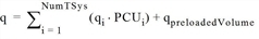
q |
Volume of a network object [car units/time interval] = sum of volumes of all PrT transport systems including base volume (preloaded volume)
|
|
qmax |
Capacity [car units/time interval] |
|
Sat |
volume/capacity ratio |
|
Fij |
Number of trips [veh/time interval] for relation from zone i to zone j. |
|
F |
Demand matrix which contains the demand for all OD pairs. |