The dynamic stochastic assignment differs from all other PrT assignment procedures as a result of the explicit modeling of the time required to complete trips in the network. For dynamic stochastic assignment - capacity has to be set as an hourly value - not regarding the length of the time interval the demand is available for.
- The dynamic stochastic assignment takes time-varying attributes of traversed links, turns, main turns and connectors into account (t0, tCur, VolCapRatio per time interval, that result from their temporary attributes, for example, Capacity and v0 or t0).
- The dynamic stochastic assignment provides the calculated results, for example volume or impedance of the connections (routes in time interval) and of their traversed network objects, which means links, turns, main turns and connectors, for each user-defined time interval. Since the impedance equals the congested travel time in most applications, time profiles for the assignment period can be generated this way. For the routes, tolls and AddValues are additionally issued for each time interval.
In contrast, all trips are completed in the case of static assignment procedures with no indication of the time required, capacities have to be specified according to the length of the time interval demand data is available for, and the volumes of all trips and the resultant impedances are superimposed upon each other at the individual network objects. Road-users subsequently only have to choose from a number of different routes for each journey. The departure time is irrelevant.
In the case of the dynamic assignment on the other hand, an assignment period T (e.g. 24 hours) is specified and divided up into time slices Ti of equal length (e.g. 15 minutes). Only the search for (alternative) routes for each journey is made with no reference to a specific time. As in the case of the static stochastic assignment, several shortest path searches are completed with network impedances that vary at random. All other operations explicitly include a time dimension. As with stochastic assignment, further random searches may be carried out (User Manual: Parameters of Dynamic stochastic assignment).
From the entire demand and its temporal distribution curve, the portion with a desired departure time is determined for each time slice within this time interval. On the supply side, there are pairs to choose consisting of route and departure time interval, which, using PuT assignment terminology, are also called connections. The impedance of a connection is composed of its network impedance and the difference between the actual and desired departure time slice (temporal utility). To determine the network impedance, the volume and the capacity-dependent travel time for each network element are stored separately for every time slice. The progress time of the trip through the network is decremented along the route, whereby for each network element the travel time of the time slice(s) in which the network element is traversed is relevant.
Image 138 shows qualitatively the procedure for calculating impedances along the time-path line of the connection.
In this case, S (= faSt) and L (= sLow) represent the capacity-dependent speed of the network element in the relevant time slice. The correct path of the trip – and thus the correct network impedance of the connection – results only when the travel time on each link (B in particular in this case) is included with respect to the time slice reached at this moment.

Image 138: Example of impedance calculation of a connection
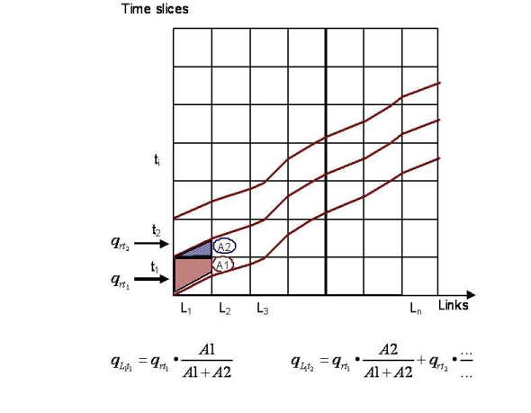
After assignment to individual connections, the network elements are loaded with the demand for each time slice as in the case of the impedance calculation, which results in new network element impedances. It is assumed that the departure times of the individual trips are equally distributed within the time slice, this means, instead of a single time-path line, a volume range is decremented (example Image 139).