To represent the spillback phenomenon, we assume that each arc is characterized by two time-varying bottlenecks, one located at the beginning and the other one located at the end, called entry capacity and exit capacity respectively.
The entry capacity, bound from above by the in-capacity, is meant to reproduce the effect of queues propagating backwards on the arc itself, which can reach the initial section and can thus induce spillback conditions on the upstream arcs. In this case the entry capacity is set to limit the current inflow at the value which keeps the number of vehicles on the arc equal to the storage capacity currently available. The latter is a function of the exit flow temporal profile, since the queue density along the arc changes dynamically in time and space accordingly with the STKW. Specifically, the space freed by vehicles exiting the arc at the head of the queue takes some time to become actually available at the tail of the queue, so that the jam density times the length is only the upper bound of the storage capacity, which can be reached only if the queue is not moving.
The exit capacity, bound from above by the out-capacity, is meant to reproduce the effect of queue spillovers propagating backwards from the downstream arcs, which may generate hypercritical flow states on the arc itself. For given arc inflows, arc outflows, and intersection priorities, which are here assumed proportional to the mid-block capacities, the exit capacities are obtained as a function of the entry capacities based on flow conservation at the node.
The network performance model is specified here as a circular chain of three models, namely the “exit flow and travel time model for time-varying capacities”, the “entry capacity model”, and the “exit capacity model”, which are solved iteratively. Image 124 shows the three models in context. The journey times which result from the solution of the three feedback model components, are combined with the monetary costs to generalized costs by an Arc Cost Model.
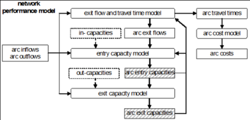
Image 124: Scheme of the fixed point formulation for the NPM
Exit flow and travel time models for time-varying exit capacity
Under the condition that the FIFO rule applies and vehicles are therefore not able to overtake, an arc performance model with time-varying exit capacity is introduced in this section. The exit flow is achieved by propagating the inflow temporal profile along the arc and thus calculating the corresponding time-series of the travel time.
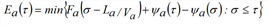
Assuming that the capacity at the end of a given edge a∈A is not reduced due to spillback effects, for a vehicle entering the edge at time τ, the hypocritical exit time ra(τ) can be expressed, dependent of the previous part of the inflow time series, which corresponds to the inflow fa(σ) at any time σ ≤ τ.
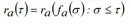
The equation [32] is described further below.
- for the trapezoidal fundamental diagram (Hypocritical exit time model for a trapezoidal fundamental diagram) (Image 123)
- for the parabolic fundamental diagram (Hypocritical exit time model for a parabolic fundamental diagram) (Image 122)
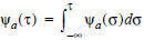
If, however, at the end of the edge there is a bottleneck with a time-varying capacity Ψa(τ) ≤ Sa for each time σ, the time series of the cumulative outflow is determined, whose value Ea(τ) at time t is defined as follows:
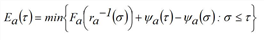
Where Ψa(τ) denotes the cumulative exit capacity at time t.
This means that Ψa(τ) - Ψa(σ) vehicles can exit the edge between times σ and τ.
The above expression [33] is based on the following specification of the FIFO rule, stating that the cumulative exit time at the exit instant ta(τ) of a vehicle that enters the arc at t is equal to the cumulative inflow at time t. This means the following:

Then, equation [33] can be explained as follows: If at a specific time t there is no congestion, the journey time is identical to the subcritical journey time, so that, based on the FIFO rule [35] the cumulative exit flow is equal to the cumulative inflow at time ra-1(τ) (a vehicle that reaches the edge at time ra-1(τ). leaves it at time t). If a queue develops at time s < t, the exit flow from this point of time to the time where the queue breaks up, then corresponds to the exit capacity. Based on the FIFO rule, this results in a cumulative exit flow Ea(τ) from the cumulative inflow at time ra-1(σ) plus the integral value of the exit capacity between σ and t, which isΨa(τ) - Ψa(σ).
By definition, the exit flow ea(τ) from arc a at time t is:
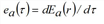
By definition, ea(τ) ≤ Ψa(τ) applies at any time τ hypercritical exit flows occur if ea(τ) = Ψa(τ).
Knowing the cumulative inflow and exit flow temporal profiles, the FIFO rule [35] yields an implicit expression for the arc exit time temporal profile.
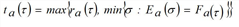
Image 125 depicts a graphical interpretation of equation [37], where the time profile of the cumulative exit flow Ea(τ) complies with the lower envelope of the following curves:
a) the cumulative inflow Fa(τ), shifted forward in time by the hypocritical travel time ra(τ) -τ thus yielding the temporal profile Fa[ra-1(τ)]. This represents the rate at which vehicles entering the arc arrive at its end.
b) for every time s, the cumulative time series of the exit capacity is shifted vertically so that it goes through the point (σ,Fa[ra-1(σ)]). This represents the rate of vehicles that can exit the arc following time s. No queue is present when curve a) prevails. Queuing starts, when the cumulative exit flow curve falls below the time-shifted cumulative entry flow curve, this means that more vehicles arrive at the final section of the arc than can exit. In the diagram, therefore, the queue arises at time s''. In Image 125, calculation of the exit time based on the cumulative time series of inflows and outflows is illustrated by thick arrows.
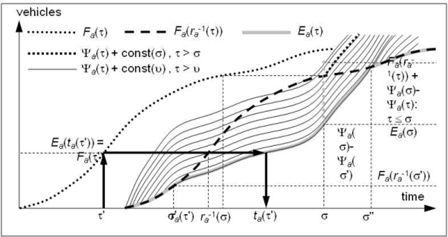
Image 125: Arc with time-varying capacity
Hypocritical exit time model for a trapezoidal fundamental diagram
If the trapezoidal fundamental diagram is adopted to represent flow states on the arc, the hypocritical speed on the link is constant, and thus equation [28] is simply specified as follows.

In this case, using [33] equation [38] can be made explicit as follows:
Hypocritical exit time model for a parabolic fundamental diagram
If the parabolic fundamental diagram is adopted, the situation becomes more complicated because vehicles may travel at different speeds even at hypocritical densities. If the arc inflow temporal profile is piecewise constant, the running link exit time can be determined at least approximately from the STKW. The general idea is to trace out the trajectory of a vehicle entering arc a at time t, observing the different speeds it will encounter along the arc, and determining its exit time ta(τ). Further below you will first find a description of the precise model. In cases where it might require large computational effort, it can be replaced by a simpler model that averages traffic conditions and thus limits the number of traffic situations encountered by vehicles on arc. Readers who would like to get a general feel for the model as a whole may just note the general idea and skip to the conclusion of this section (Input and output attributes of dynamic user equilibrium).
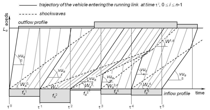
Image 126: Flow pattern given by the Simplified Theory of Kinematic Waves
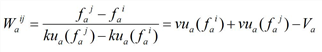
Based on the STKW, vehicles change their speeds instantaneously. As depicted in Image 126, when the inflow temporal profile is piecewise constant, vehicle trajectories are piecewise linear. Furthermore, the space-time plane comes out to be subdivided into flow regions characterized by homogeneous flow states and delimited by linear shock waves. The slope Waij of the shockwave separating the two hypocritical flow states Φ(fai) and Φ(faj) is:
In theory, given a piece-wise constant inflow time series, it is possible to determine the trajectory of a vehicle entering the arc at instant t, and thus its hypocritical exit time ra(τ). The Image 126 shows that it may actually be extremely cumbersome to determine these trajectories.
- Many shockwaves may be active on the arc at the same time.
- Shockwaves may be generated either at the initial section by flow discontinuities at times τi, 0 ≤ i ≤ n-1, or by shockwave intersections on any arc section at any time.
- A vehicle may cross many shockwaves while traveling on the arc, and all the crossing points have to be explicitly evaluated in order to determine its trajectory.
In order to overcome these difficulties, as depicted in Image 127, we assume that at each instant ri, 0 ≤ i ≤ n-1, a fictitious shockwave is generated on the initial arc section separating the actual flow state Φ(fai+1) from a region with the average speed λi = L / (rai - τi) of the vehicle that reaches the arc at time τi.
Fictitious shockwaves are very easy to deal with due to the following reasons:
- They never touch each other and are therefore all generated on the current initial link section only at time τi, 0 ≤ i ≤ n-1.
- Each vehicle meets at the most the last generated fictitious shockwave, so that its trajectory is very easy to be determined.
Based on [36], slope Wai of the fictitious shockwave is as follows:
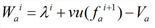
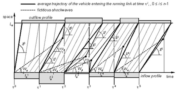
Image 127: Flow pattern given by the Averaged Kinematic Wave model
Note that the trajectory of a vehicle entering the current link at time τ∈(τi-1,τi] is directly influenced only by the mean trajectory of the vehicle entered at time τi-1, summarizing the previous history of flow states on the arc.
The approximation introduced has little effect on the model efficacy. Moreover, it satisfies the FIFO rule, which is still ensured between the arc initial and final sections, while local violations that may occur within intermediate sections are of no interest.
Based on the above, the hypocritical travel time τai = τa(τ)i, 0 ≤ i ≤ n-1 can be specified as follows:
a) If a vehicle entered at time τi does not meet the fictitious shockwave Wai-1 before the end of the arc, its hypocritical exit time is simply:
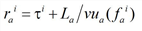
Here, fai is the arc inflow during time interval (τi-1,τi].
b) Otherwise, its hypocritical exit time is determined on the basis of the two speeds it assumes before and after crossing the fictitious shockwave.
where ωi is the travel time of the vehicle before it reaches the fictitious shockwave (Image 128).
Image 128: Determination of the arc hypocritical exit time
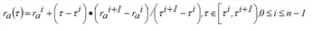
Then, the hypocritical travel time ra(τ) specifying [32] is:
Entry capacity model
In this section we propose a new approach to represent the effect on the entry capacity of queues that, generated on the arc final section by the exit capacity, reach the arc initial section, thus inducing spillback conditions. This part of the model is used only if DUE is run with the spillback option activated (User Manual: Blocking back model settings and calculation). If the option is turned off, the storage capacity of an arc is assumed to be infinite, and the entry capacity of a link is never reduced below the in-capacity.
To help understand let us assume, for the moment, that the queue is uncompressible, that means, only one hypercritical density exists. Then, the kinematic wave speed is infinitive – from either Image 122 or Image 123 it is clear that wa = ∞ with KJa = k2a – so that any hypercritical flow state occurring at the final section would back-propagate instantaneously. This circumstance does not imply that the queue reaches the initial section instantaneously. There, the exiting hypercritical flow state does actually not affect the entering hypocritical flow state until the arc has filled up completely. This means, that the cumulative number of vehicles that have entered the arc equals the number of vehicles that have exited the arc plus the storage capacity. The latter in this case is constant in time and given by the arc length multiplied by the maximum queue density. As soon as the queue exceeds the arc length, the entry capacity becomes equal to the exit capacity, that means, all vehicles on the arc move as one rigid object.
In reality, hypercritical flow states may actually occur at different densities. Their kinematic wave speeds are not only lower than v0, implying that the vehicles will reach the first arc section with a delay when starting from the final section, but also somewhat different from each other, which generates a distortion in their forward propagation in time. Notice that the fundamental diagrams adopted here are capable of representing the dominant delay effects but not the distortion effects, since all backward kinematic waves have the same slope.
The spillback effect on the entry capacity is investigated by exploiting the analytical solution of the STKW. The flow state occurring on an arc section is the result of the interaction among hypocritical flow states coming from upstream and hypercritical flow states coming from downstream. Specifically, on the initial section, the one flow state coming from upstream is the inflow, while the flow states coming from downstream are due to the exit capacity and can be determined by back-propagating the hypercritical portion of the cumulative exit flow temporal profile, thus yielding what we refer to as the “maximum cumulative inflow” temporal profile.
According to the Newell-Luke minimum principle, the flow state consistent with the spillback phenomenon occurring at the initial section is the one implying the lowest cumulative flow. Therefore, when the cumulative inflow equals or overcomes the maximum cumulative inflow, so that spillback actually occurs, the derivative of the latter temporal profile may be interpreted as an upper bound to the inflow. This enables the determination of the proper value of the entry capacity that maintains the queue length equal to the arc length.
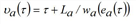
The instant υa(τ) when the backward kinematic wave generated at time t on the final section of arc a∈A by the hypercritical exit flow ea(τ) = Ψa(τ) would reach the initial section is given as follows.
By definition the points in time and space constituting the straight line trajectory produced by a kinematic wave are characterized by a same flow state. Moreover, Image 129 shows that the number of vehicles encountered by the hypercritical wave relative to the exit flow q for any infinitesimal space ds traveled in the opposite direction is equal to the time interval ds  multiplied by that flow. Therefore, integrating along the arc from the final to the initial section, we obtain the maximum cumulative flow Ha(τ) that would be observed at time υa(τ) in the initial section as:

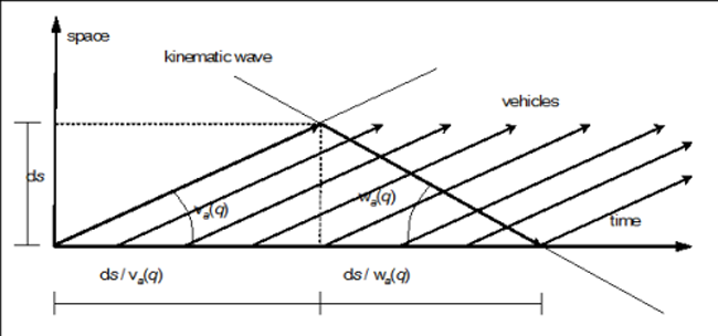
Image 129: Trajectories of a hypercritical kinematic wave and of the intersecting vehicles
In the fundamental diagrams adopted here, the hypercritical branch is linear and therefore υa(τ) is invertible. Since wa(q) = wa is the time at υa(τ) = τ, based on [43], σ = τ - La /wa. Furthermore, Ha(τ) = Ea(τ) + La • KJa results, based on [44] q/va(q) = KJa - q/wa. Therefore, the maximum cumulative inflow Ga(τ) that could have entered the arc at time t due to the inflow volume is given by the following equation:
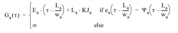
If the cumulative inflow Fa(τ) at time t equals or exceeds the maximum cumulative inflow Ga(τ), so that spillback occurs at that instant, then the entry capacity μa(τ) is given by the derivative dGa(t)/dτ of the latter; otherwise, it is equal to the in-capacity Qa.
Differentiating Ga(τ) implies the following:
 =
= 
From ea(τ - La /wa), the following applies:
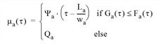
Image 130 shows how, based on equation [45], the time series of the maximum cumulative inflow can be obtained graphically through a rigid translation (thick arrows) of the cumulative exit flow time series for La / wa in time and for La • KJa in value. Moreover, it points out that if Ga(τ) is greater than Fa(τ), the queue is shorter than La and μa(τ) = Qa.
Otherwise spillback occurs and μa(τ) = Ψa(τ - La /wa).
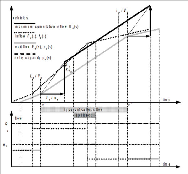
Image 130: Graphical determination of the time series of the inflow capacity in the case of triangular fundamental diagram, piecewise constant inflow, and constant exit capacity
Exit capacity model
In this section we present a model to determine, for a given node, the exit capacities of the upstream arcs, on the basis of the entry capacities of the downstream arcs and of the turn volumes. Only two node forms occur in the graph that is formed on the basis of the Visum network. These are joining links and diverging links. In this case, the model can be described by the inflows and outflows of edges.
When considering joining links x∈N, that is an intersection with a singleton forward edge, the problem is to split the entry capacity μb(τ) of the edge b = FS(x) available at time t among the edges belonging to its backward edge, whose outflows compete to get through the intersection. In principle, we assume that the available capacity is distributed proportionally to the out-capacity Sa of each arc a∈BS(x). But this way it may happen that on some arc a the outflow μa(τ) is lower than the share of entry capacity assigned to it, so that only a lesser portion of the latter is actually exploited. The rest of the entry capacity is then partitioned among the other arcs. Moreover, when no spillback phenomenon is active, the exit capacity Ψa(τ) is set equal to the out-capacity Sa.
When considering diverging links x∈N , that is an intersection with a single backward edge, the exit flow of this edge a = BS(x) is determined by the most restrictive entry capacity among the forward edges. If no arc is spilling back, the exit capacity is set equal to the out-capacity. If only one arc b∈FS(x)is spilling back, that is fb(τ) ≥ μb(τ), then the exit capacity μa(τ), scaled by the share of vehicles turning on arc b is set equal to the entry capacity of b in order to ensure capacity conservation at the node while satisfying the FIFO rule Ψa(τ) • fb(τ) / μa(τ) = μb(τ) applied to the vehicles exiting from arc a. If more than one arc b∈FS(x) is spilling back, the exit capacity is the most penalizing among the above values. On this basis, the following equation is derived:

Note that, in contrast with the models presented in the previous two sections, this model is spatially non-separable, because the exit capacities of all the arcs belonging to the backward star of a same node are determined jointly, and temporally separable, because all relations refer to a same instant.
It is assumed that vehicles do not occupy the intersection if they cannot cross it due to the presence of a queue on their successive arc, but wait until the necessary space becomes available. Indeed, this model is not capable of addressing the deterioration of performances due to a misusage of the intersection capacity.
Arc Cost Model
The cost for vehicles entering arc a at time t is given as follows:
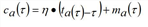
Here, ma(τ) describes the monetary costs, and η represents the value of time.
