As the analysis is carried out within a dynamic context, the model variables are temporal profiles, here represented as piecewise continuous functions of the time variable t.
Users trips on the road network are modeled through a strongly connected oriented graph G = (N, A), where N is the set of the nodes and A ⊆ N ´ N is the set of the arcs. Each link, turn, and connector in the Visum network corresponds to an arc. Each Visum network node and zone corresponds with a node from G.
Each arc a is identified by its start node (FromNode) TL(a) and by its end node (ToNode) HD(a).
Thus a = (TL(a), HD(a)).
Example
For an arc a representing a link in the Visum network, TL(a) would correspond to its From-node and HD(a) to its To-node. The forward and backward star of node x∈N are denoted, respectively, FS(x) ={a∈A: x = TL(a)} and BS(y) = {aÎA: y = HD(a)}. The zones constitute a subset Z ⊆ N of nodes.
When traveling from a node o∈N to a node d∈Z users consider the set Kod of all the paths connecting o and d on G. The focus is on the n:1 shortest path problem from each node o∈N to a given destination d∈Z. It is assumed that graph G is strongly connected, so that Kxd with x∈N ≠ d∈Z is not empty.
Path topology is described through the following set notation:
A(k) = concatenated sequence of arcs constituting the path k∈Kod from o∈N to d∈Z.
The following notations are adopted for the network volumes.
|
Dod(τ) |
Demand of vehicles, which are moving from origin o∈N to destination d∈Z and are departing at time τ |
|
fa(τ) |
Flow of vehicles, which at time τ are traversing arc a∈A |
|
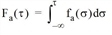
Fa(τ) |
Cumulated flow of vehicles, which at time τ are traversing arc a∈A |
|
ua(τ) |
Exit flow from arc a∈A at time τ |
The following applies by definition:
For the calculation of network performance, travel times are introduced through inflow-outflow functions, and the following notation is adopted.
|
ca(τ) |
Cost of traversing arc a∈A for vehicles entering it at time τ |
|
ta(τ) |
Outflow time of arc a∈A for vehicles entering it at time τ |
|
fa-1(τ) |
Inflow time of arc a∈A for vehicles exiting it at time τ |
|
Ck(τ) |
Cost of path k∈Kod from o∈N to d∈Z for vehicles departing from node o at time τ |
|
Tk(τ) |
Outflow time of path k∈Kod from o∈N to d∈Z for vehicles departing from o at time τ |
Due to the presence of time-varying costs, it may be convenient to wait at nodes in order to enter a given arc later. In the following, it is assumed that vehicles are not allowed to wait at nodes, but instead paths with cycles may seem the better option. However, the shortest paths include at most a finite number of cycles.
Since waiting at nodes is not allowed, the path exit time Tk(τ) is the sum of the travel times of its arcs A(k), each of them referred to the instant when these vehicles enter the arc when traveling along the path. Moreover, assuming that path costs are additive with respect to arc costs, its cost Ck(τ) is the sum of the costs of its arcs A(k). The outflow time or the cost, respectively, of path k can then be retrieved through the following recursive equations:

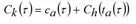
where a = (o, x)∈A is the first arc of k and h∈Kxd is the remainder of path k (Image 121).
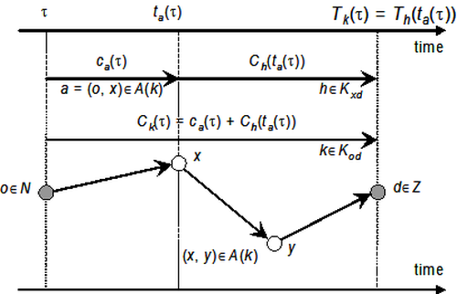
Image 121: Recursive expressions of path exit time, entrance time and cost
The strict First In First Out (FIFO) rule holds if the following property is satisfied for each arc a∈A:
 , for all
 The monotonicity expressed by [30] ensures that the temporal profiles of the arc exit times are invertible. Moreover, the FIFO rule applies also to the entrance times.
 , for all
 Any arc a∈A consists of a homogeneous channel with two bottlenecks located at the beginning and at the end. The flow states along the arc are determined on the basis of the Simplified Theory of Kinematic Waves (STKW), assuming the concave parabolic-trapezoidal fundamental diagram depicted in Image 122, expressing the vehicle flow qa(x,τ) at a given section x of the arc and instant t, as a function of vehicle density ka(x,τ) at the same section and instant.
The arc is then characterized by:
|
La |
Length of arc a |
|
Qa |
Capacity of the initial bottleneck and of the homogeneous channel associated with arc a, called in-capacity; |
|
Sa |
Capacity of the final bottleneck associated to arc a, simulating the average effect of capacity reductions at road intersections (i.e. due to the presence of signal controllers), called out-capacity Sa ≤ Qa; |
|
Va |
Maximum speed allowed on arc a, called free flow speed in Visum |
|
KJa |
Maximum density on arc a called jam density |
|
Wa |
propagation speed of hypercritical flow states on arc a, called hypercritical kinematic wave speed. |
Within this framework, for links the in-capacity corresponds to the physical mid-block capacity, whereas out-capacity reflects the bottleneck capacity imposed by the signal controller or priority rules at the downstream junction. Exit connectors (x, d)∈A: x∈N \ Z, d∈Z are arcs with infinite in-capacity, entry connectors (o, y)∈A: o∈Z, y∈N \ Z are arcs with infinite out-capacity. Turns, however, are represented by arcs having zero length and in-capacity equal to their out-capacity.
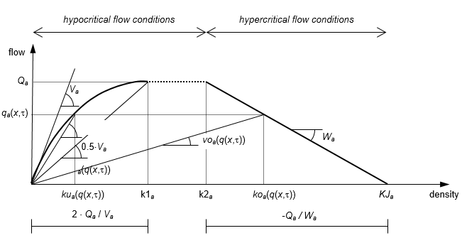
Image 122: The adopted parabolic-trapezoidal fundamental diagram, expressing the relation among vehicular flow, speed, and density along a given arc.
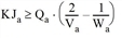
In Image 122, k2a ≥ k1a is assumed, implying the following relation among the above parameters:
Based on the fundamental diagram, it is possible to identify two families of flow states.
- Hypocritical flow conditions corresponding to uncongested or slightly congested traffic. Under these conditions, if vehicular density increases, the vehicular flow increases also.
- Hypercritical flow conditions corresponding to heavily congested traffic. Queues and “stop and go” phenomena occur. Under these conditions, if vehicular density increases, the vehicular flow decreases.
Then, koa(q) and voa(q) express the density and the speed as functions of the flow in presence of hypercritical flow conditions, while kua(q) and vua(q) express the density and the speed as functions of the flow in presence of hypocritical flow conditions.
When modeling arcs with low speed limits, i.e. representing urban roads, it may be assumed that the vehicle speed under hypocritical flow conditions is constant and equal to the speed limit, until capacity is reached. In this case, the simpler trapezoidal fundamental diagram depicted in Image 123 may be adopted, whereby in order to guarantee k2a ≥ k1a, the following relation must apply:
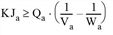
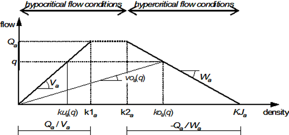
Image 123: The trapezoidal fundamental diagram suggested for urban links
In order to implement the proposed models, the period of analysis [0, Q] is divided into n time intervals identified by the sequence of instants τ= {τ0, … , τi, … , τn},with τ0 = 0, τi < τj for all 0 ≤ i < j ≤ n, and τn= Q. For computational convenience, we introduce also an additional instant τn+1= ∞.
In the following we approximate the temporal profile g(τ) of any variable through either a piecewise linear or a piecewise constant function, defined by the values gi = g(τi) taken at each instant τi∈τ. This way, any temporal profile g(τ) can be then represented numerically through the vector g = (g0, … , gi, … , gn).
