Defining the Wiedemann 99 model parameters
This model is based on Wiedemann’s 1999 car following model.
The following parameters are available:
| Parameters | Unit | Description |
|---|---|---|
|
CC0 |
m |
Standstill distance: The desired standstill distance between two vehicles. No stochastic variation. You can define the behavior upstream of static obstacles via the attribute Standstill distance in front of static obstacles (Editing the driving behavior parameter Following behavior). |
|
CC1 |
s |
Gap time distribution: Time distribution from which the gap time in seconds is drawn which a driver wants to maintain in addition to the standstill distance. At a speed v the desired safety distance is computed as: dxsafe = CC0 + CC1 • v At high volumes this distribution is the dominant factor for the capacity. |
|
CC2 |
m |
'Following' distance oscillation: Maximum additional distance beyond the desired safety distance accepted by a driver following another vehicle before intentionally moving closer. If this value is set to e.g. 10 m, the distance oscillates between: dxsafe und dxsafe + 10 m The default value is 4.0m which results in a quite stable following behavior. |
|
CC3 |
s |
Threshold for entering ‘BrakeBX’: Time in seconds before reaching the maximum safety distance (assuming constant speed) to a leading slower vehicle at the beginning of the deceleration process (negative value). |
|
CC4 |
m/s |
Negative speed difference: Lower threshold for relative speed compared to slower leading vehicle during the following process (negative value). Lower absolute values result in adopting a speed more similar to the leading vehicle. |
|
CC5 |
m/s |
Positive speed difference: Relative speed limit compared to faster leading vehicle during the following process (positive value). Recommended value: Absolute value of CC4 Negative values result in adopting a deceleration speed more similar to the leading vehicle. |
|
CC6 |
1/(m • s) |
Distance impact on oscillation: Impact of distance on limits of relative speed during following process:
|
|
CC7 |
m/s2 |
Oscillation acceleration: Acceleration oscillation during the following process. |
|
CC8 |
m/s2 |
Acceleration from standstill: Acceleration when starting from standstill. Is limited by the desired and maximum acceleration functions assigned to the vehicle type. |
|
CC9 |
m/s2 |
Acceleration at 80 km/h: Acceleration at 80 km/h is limited by the desired and maximum acceleration functions assigned to the vehicle type. |
|
|
Notes:
The following applies to cars only: z is added to the maximum acceleration used: z = value from the interval [0.1], normally distributed by 0.5 with a standard deviation of 0.15. The acceleration of the vehicle may be less than its maximum acceleration if other factors are involved, for example if the vehicle is very close to its desired speed or if it perceives a slower vehicle in front.
|

Defining the saturation flow rate with the Wiedemann 99 modeling parameters
The saturation flow rate defines the number of vehicles that can flow freely on a link for an hour. Impacts created through signal controls or queues are not accounted for. The saturation flow rate also depends on additional parameters, e.g. speed, share of HGV, or number of lanes.
In the car-following model Wiedemann 99, parameter CC1 has a major impact on the safety distance and saturation flow rate. The scenarios shown below as an example are based on the following assumptions:
- car-following model Wiedemann 99, containing default parameters with the exception of CC1 that varies across the x-axis
- one time step per simulation second
The main properties of the following graphs are:
|
Scenario |
Right-side rule |
Lane |
Speed cars* |
Speed HGV* |
% HGV |
|---|---|---|---|---|---|
|
99-1 |
no |
2 |
80 |
n/a |
0% |
|
99-2 |
no |
2 |
80 |
85 |
15% |
|
99-3 |
yes |
2 |
80 |
n/a |
0% |
|
99-4 |
yes |
2 |
80 |
85 |
15% |
|
99-5 |
yes |
2** |
120 |
n/a |
0% |
|
99-6 |
yes |
2 |
120 |
85 |
15% |
* Vissim default setting
** Lane 2 closed for HGV traffic
|
|
Note: The graphs show exemplary calculated saturation flow rates. When using a different network, you receive graphs depicting different values. |
Example: Graphs of saturation flow rate Scenario 99-1 to 99-6
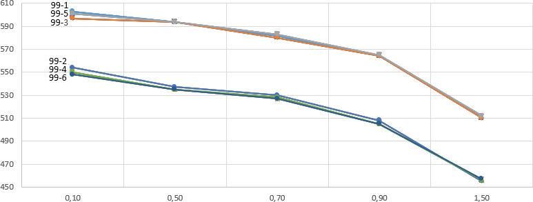
Horizontal x-axis: Variation CC1: 0.1 to 1.5
Vertical y-axis: Veh/h/lane
Superordinate topic:
