TRE (support issues)

The parameter fore represents the time span in seconds between:

• The time of the forecast (time when the simulation was started)
• The current time

So, for example, results with a value of fore = −900 are from the previous 15 minutes.

TRE is a rolling simulation. It takes the previous slice as a starting point to run the simulation, so:

• You can see the results for fore = −900 as a picture of how the reality was.
• You can see any value of fore >= 0 as a simulation of the future state of the traffic network.

Sometimes you might get a number of warning messages about some demand not being loaded. (Example: Demand from origin -1 to destination -2 is not connected and will not be loaded.)

These messages are due to the fact that no route has been found from the origin to the destination. Sometimes this is related to the disconnection of connectors on nodes with geometry. Due to confusion in case of nodes with signals and connectors, TRE does not allow to turn from or to connectors if a geometry is present on the node.

A workaround is to disable the geometry of all nodes with connectors:

1. Create a filter on nodes that have connectors.
2. Right-click the node layer.
3. Multi-edit.
4. Click the Special functions tab.
5. Select Only active ones.
6. Choose the function Lane definition.
7. Click the Reset lane data button.

This resets the geometry for all nodes with connectors and allows to use connectors.

Note that this:

• Does not allow to model approach lanes in a number different from the link lanes (Link.NumLanes)
• Does not allow to signalize these nodes

TRE in off-line mode performs Dynamic User Equilibrium. The dynamic assignment algorithm uses an iterative procedure called Trajectory Dynamic Traffic Assignment (dta) with MSA.

The default stop criteria are either 100 iterations or an acceptance gap among successive steps equal to 1e-6. The default configuration of TRE does not use the Gradient Projection approach.

The OD matrices of the base model were calibrated with an OD matrix correction procedure (TFlowFuzzy implemented in PTV Visum) using:

• a set of historical traffic counts

• a set of seed OD matrices (taken from the original model)

• a set of path flows (estimated with the traffic assignment)

Since the seed matrices were taken from an existing transport model of the base model, we can assume that the OD matrix correction procedure has improved the seed matrices only slightly.

When a set of detected trajectories will be available in the study area, it will be possible to validate the new corrected OD matrices and the path flows with observed data.

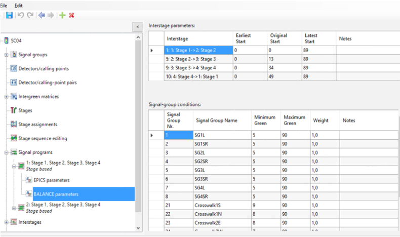
The weights are supplied at each signal group in the software Vissig.

The standard weight is 1, but it can be changed during the calibration phase. Take a look at the screenshot below to see where this is done in the program.

Visum read the original description of the network model and provide the rendering of the node geometry, both for:

• Nodes
• Main Nodes

If you change some element of the geometry, the property DefNodeGeometry is set to False:

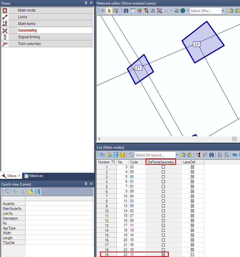
TRE ignores the geometry for:

• Nodes contained into a Main Node.
• Nodes (or Main Nodes) with DefNodeGeometry = True (see the check-box associated to the Main Node 23).

Run a DTA twice with the same settings but two different durations, for example:

• First run based on 8-10 AM
• Second run based on 8-12 AM

Now you can isolate a common time interval, for example the interval 9:45 AM-9:50 AM.

In this case, you could get different assignment results, for example different entry flows during the interval.

Tip:  The issue does not apply in the methodology implemented in the new Temporal Layer DTA.

This result could be consistent with the methodology of the Trajectory-based DTA and some possible distortions in the paths.

The amount of “unreliable” DTA intervals, starting from the last, is smaller the shorter (in time) are the DTA paths.

This approximation can be avoided with advanced options of the TRE algorithm.

Option 1

You can act on the parameter DtaSpan (see → Equilibrium parameters > DtaSpan).

The strategy is based on setting the simulation end time after the demand end time.

The general relation could be described as:

Simulation_ENDTIME = Demand_ENDTIME + DELTA

DELTA is a value (in seconds) >0 and its right value can vary and must be determined according to a lot of factors (mainly, the dimension of the network model and associated attributes).

Option 2

Another option is to set the simulation end later than the end of the demand time series. Creation of empty matrices is not needed. The required additional simulated time is longer the longer (in time) are DTA paths

Sometime you can observe some discrepancy between TRE results compared with some attributes value model based.

Limitations of the model about speed and travel time

A specific limitation is related to the average speed forecast multiplied by the link travel time forecast yield much longer distances than the relevant link's actual length:

SPED x TIME = LENGTH

Where:

• SPED = RLIN_TSYS_TRE_*.SPED
• TIME = RLIN_TSYS_TRE_*.TIME
• LENGTH = LINK.LENG

The reason about this unexpectd result can be explained considering that the link average speed over a result interval (SPED) could not be consistent with the travel time (TIME) given for the same interval.

The average speed is calculated from flow states on the link fundamental diagram (by network model), and accounts for many corrections including speed and flow measures on any of the underlying streets.

The travel time is calculated from flow cumulatives according to the First In - First Out rule, and for each simulation interval it is relevant only to the vehicle entering the link in its final instant (instant measure).

A speed measure can be higher than the link speed limit, and can be extended onto the next interval (in the future), while travel times for that interval reflect the propagation speeds given by the model, unaffected by the measure projection.

Limitations of the model about events

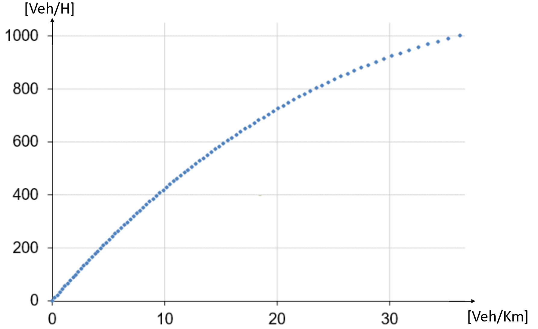
In the model of the propagation of flows based on TRE engine, a traffic state is generally identified by the couple:

• Flow, measured in [Veh/H].
• Density, measuered in [Veh/Km].

The traffic states belongs to the Fundamental Diagram (FD) curve (→ Speed measure effects).

In the figure, the Hypocritical section of the FD:

In such cases, TRE produces forecast traffic state points not belonging to the diagram (inconsistent traffic states), as shown through the set of green points in the figure:

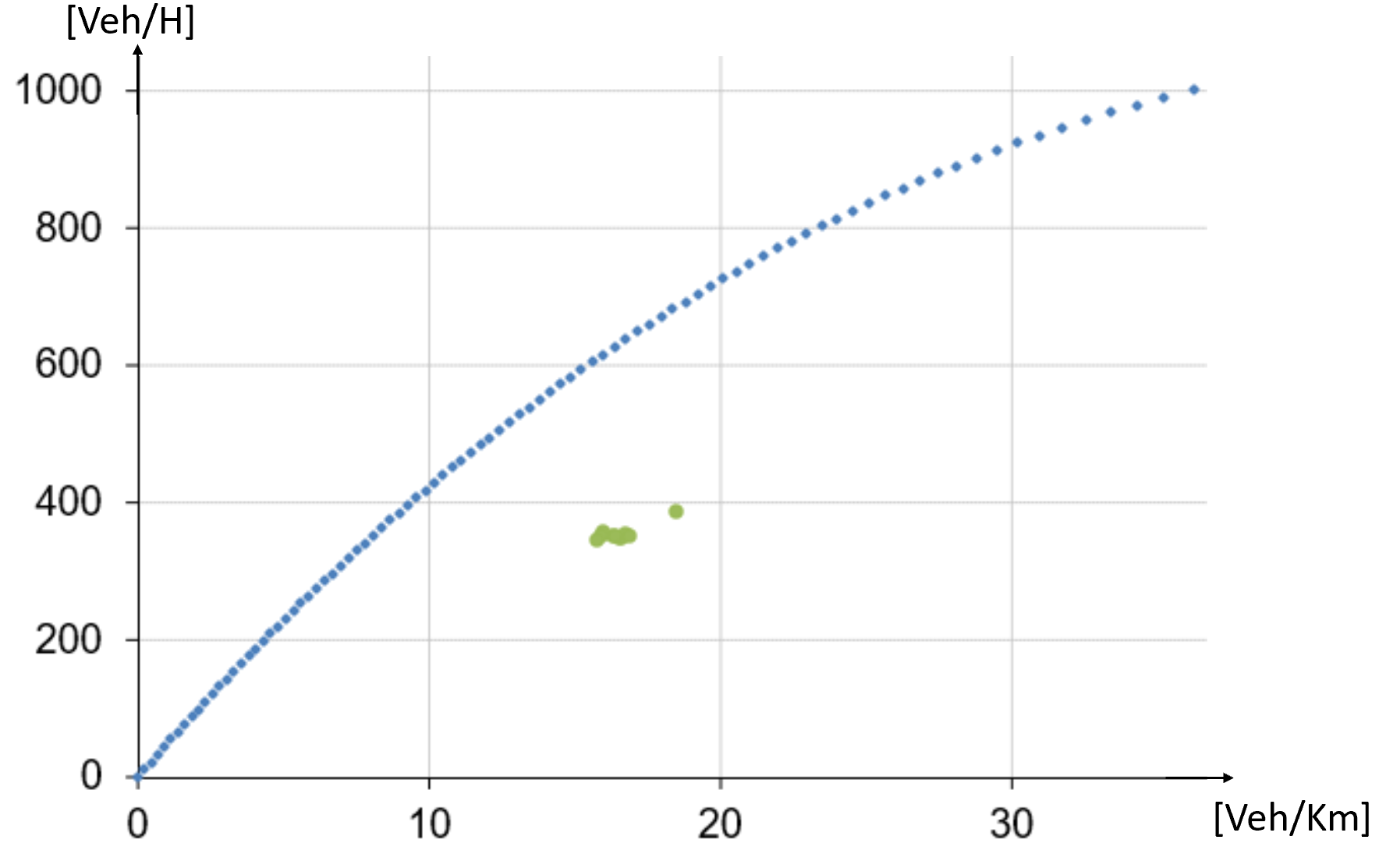
The situation is associated to the presence of specific events:

• Capacity reduction event.
• Speed reduction event.

If one or both events are present on a specific link, TRE modifies the FD associated to the link, as qualitatively shown in the figure:

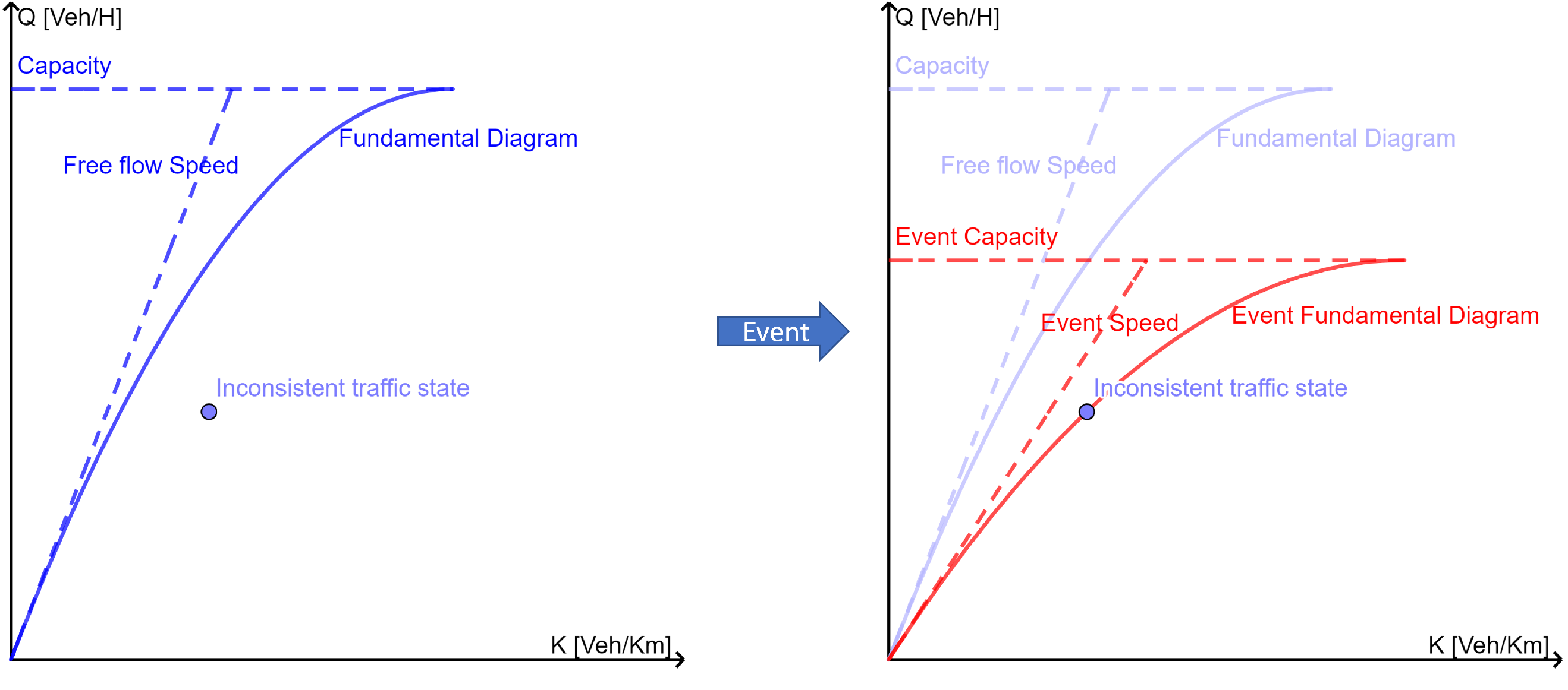
The tangent line to the fundamental diagram at the point (0,0) represents the velocity at zero flow. When TRE receives an event, the slope of the line changes.

In the figure you see an event of capacity reduction, represented by the horizontal red-dashed line.

The slope of the FD changes (red curve); the previous inconsistent traffic state belong to the new Event Fundamental Diagram curve.

Travel Time and Simulation Time: effects of the NormalizeDistortedResults parameter

In TRE, for every link, there is a model constraint for which the link travel time can not be less than the simulation time period:

L=>V X tt_j

tt_j=> tt_sim

Parameter	Description
L	The length of the link.
V	The link free flow speed.
ttj	Travel time associated to the link j.
ttsim	The simulation time period.

Example

Parameter	Description
L	100 m
V	10 m/s
ttj	10 s
ttsim	20 s

With tt_j< tt_sim, the constraint is violated.

You can provide a remediation in two ways:

• Set L=200 m and maintain V=10 m/s (if → StretchArcs=true).
• Set V=5 m/s and maintain L=100 m (if → StretchArcs=false).

In both cases tt_j=tt_sim.

Important:  The possible violation of the constraint can happens for every link of the network. Therefore, for every link could be necessary to provide such remediation.

The indicated remediations are based on a scalar value K>0.

In the example, K=2 for L or K=0.5 for V.

The value K has an impact on other variables associated to the link, as shown in the table:

L	Description	V	Description
STOR	Storage capacity of the link.	SPED	Speed.
NVEH	Number of vehicles.	TIME	Travel time.
QUEU	Number of vehicles in the queue.
QUEN	Share of queuing vehicles.
QUEL	Contains the ratio between the length of the queue and the length of the link. If QUEL = 0.66, the length of the queue cover the 66% of the link length.
TIME	Travel time.

The scalar factor K is used, during the simulation, to maintain the constraint set by simulation time period. At the end of the simulation, the calculated values are stored in the DB; before storing it, the values must be scaled of the K factor (→ NormalizeDistortedResults).

Important:  Not all results can be back-normalized.

The result of this process can imply some inconsistencies.

Example: output vehicles from a queue larger than the queue itself

In a link where the length L has been doubled (K=2), which contains, at a certain time, a certain number of vehicles in the queue, this number is equal to half the number defined in the simulation.

But the number of vehicles that leave the link is the same as in the simulation.

The inconsistency between the vehicles present on the link and those leaving it depends on the mechanism associated with the scalar factor K (OFLW).

Example: outflow starts later than travel time

In a link where the length L has been doubled (K=2), the travel time is half the number defined in the simulation.

But the vehicles leave the link after a time equal to the simulation time.

The inconsistency between the travel time and the instant in which the vehicles leave (OFLW).

As from GLTM methodology (see → General Link Transmission Model (GLTM)), links cannot be run by waves faster than a simulation clock (SimIntD).

TRE initially compares SimIntD with the ratio between the link length and the faster between its free-flow speed (SPED (V0PrT in Visum)) and hypercritical wave speed (JWAV (DUEvWave in Visum)).

If SimIntD is longer, the links too short are internally stretched.

TRE sets the link lengths based on static input attributes:

• Free-flow speed.
• Hypercritical wave speed.

It can happen (for the free-flow speed) that a measurement or an event tries to set it to a too high value for the link length.

In the figure (Traffic Supervisor GUI), we can see a road with:

Free-flow speed = 20 km/h

Link length = 73 m

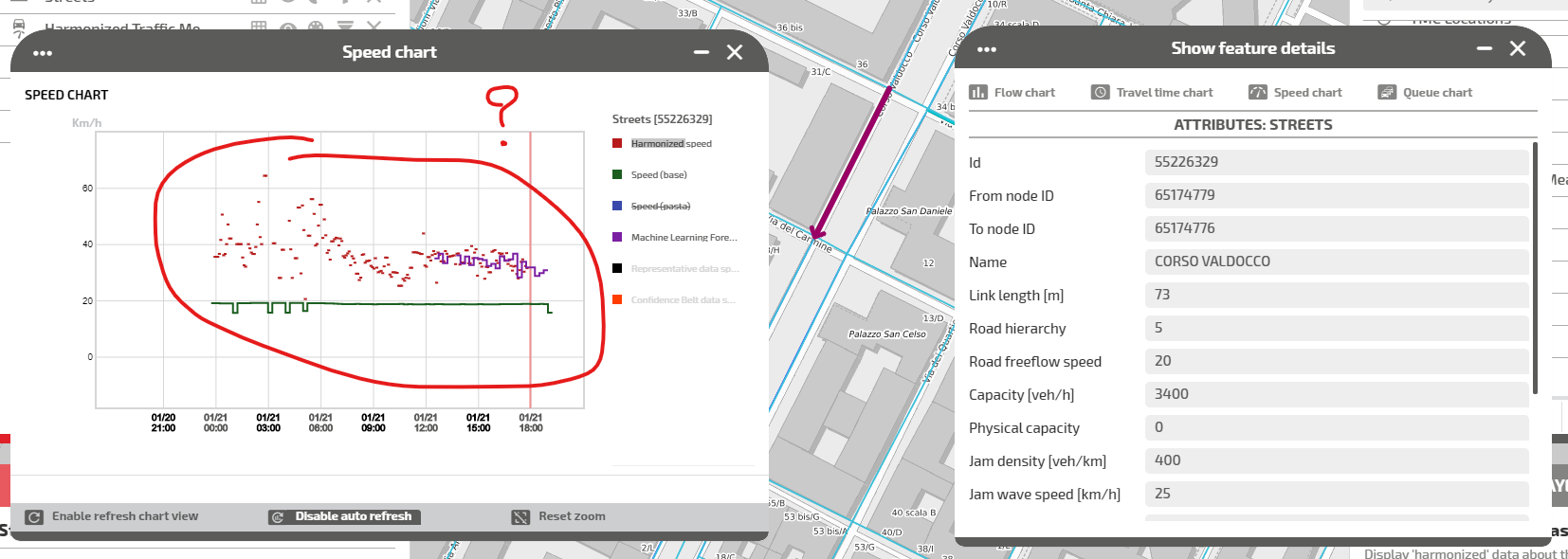
TRE results does not match neither the ML forecast, nor the harmonized measurements, because the link is short.

The free flow travel time is:

73/20*3.6 = 13.14 s

With SimIntD of 12 seconds, the maximum speed measure is:

73*3.6/12 = 21 km/h > Free-flow speed

In this case, possible remediations are:

• Increasing free-flow speed of the link.
• Decreasing SimIntD.
• Increasing link length.

In case no day-type was found with assignment done (see Layout_Validities>dtyp and Layout_Model_Simulation>tprb) , an error message is stored into TRE log file:

Demand activation day-type not found for simulation date [dd/MM/yyyy]:
possibly, no day-type found with equilibrium_computed = True or with available TPRB

If multiple installations of TRE are present in the system, they may have access to different turn borbability sources for different day types.

In such case, a conflict is generated and the value of the column equilibrium_computed may be consistent with only one of the TRE installation.

Important:  For avoiding the conflict, it is important to check that all the TRE instance have the same turn probabilities source (binary files or database table).

TRE presents a "false bug" that apparently consists of a gap between:

• The measured flow.
• The simulated outflow at forecast distance zero.

At forecast distance zero, no difference is expected.

Additionally, these "false bug" occurs only on few links.

The issue is based on two factors:

1. The link has a geometry (lanes).
2. The link head is on a signalized intersection.

The link has a geometry (lanes)

The flow measure is applied on the head of the link trunk. Since the propagation on the lanes is not instantaneous, the average outflow in the result interval can not be exactly consistent with a measure starting at the beginning of that interval.

The link head is on a signalized intersection.

There is some capacity reduction on the head of the lanes (actually on the turns exiting from the lanes). The capacity reduction is not overridden by the flow measure, since the measure itself is applied on the link trunk.

The evidences observed (→ List of datasources) are:

• Disabling the signals datasource (DS_SIGN=-2), the gap is greatly reduced (<10 [veh/h]).
• Disabling the junction datasource (DS_JUNC=-2) the gap becomes zero.

TRE presents, in some cases, link results with very small speed values, but different from zero.

The reason of these results is associated to two specific conditions:

• Hypercritical speed measurements together with small flow measurements
• HypercriticalSpeedMeasureSetQueue = false (→ Traffic data parameters)

To match the measure, is used the Fundamental Diagram Correction (FCF) algorithm (→ Speed measure effects > Fundamental Diagram Correction (FDC)).

The algorithm present some intrinsic well known limitations and it can fails.

The solution is to set:

HypercriticalSpeedMeasureSetQueue = true

The TRE simulation engine provides simulations of the behavior of the traffic network based on simulation periods of 15 minutes.

TRE calculates:

• The speed on a link considering the average density of vehicles on the link and interpolating the speed value from the fundamental diagram.
• The travel time on the link is the instantaneous travel time corresponding at the final instant of the simulation interval considered.

It's almost evident that these two traffic parameters are calculated in a very different way and they can not be considered as "homogenous" values.

For this reason, is misleading to compare the path travel time as computed by the procedures:

• The sum of the instantaneous travel time of all links of the path.
• The sum of the ratio between the length of a link and the speed computed by TRE, for all the links of the path.

Optima provides a specific KPI (→ KPI templates > Path Travel Time - Provider: Short-Term Forecast).

TRE offline usually automatically calls the latest registered version of Visum through the Visum.Visum COM key. If you wish to register, and therefore, utilize a different version of Visum, follow these steps:

1. Open the Visum version you would like to use

2. Run Help > Register as COM server.

The Visum.Visum COM key is now overwritten with your chosen Visum version, and TRE offline will now automatically call it.