Destination and mode choices for activity executions and trips of a tour are made sequentially, with a choice always based on previous choices. Here, the so-called main activity, i.e. the central activity, begins. Then the destination and mode of the subsequent (secondary) activities are determined one after the other.
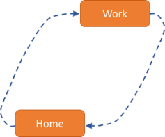
Thus, in a trip chain such as Home - Work - Shopping - Home, the destination of the work activity is chosen first. For each choice, the utilities of the entire (previously calculated) trip chain are always taken into account. In tour-based models, this principle is called rubberbanding. Since only the home locations are known in the first step, the trip chain Home - Work - Home is considered, whereby the utilities of the trips Home - Work and Work - Home are included in the choice.

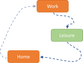
In the next step, the leisure location is selected, i.e. the trip chain Home - Work - Leisure - Home as well as the trips Work - Leisure and Leisure - Home are considered (the trip Home - Work is already determined and is therefore not considered further).

At each step, the destination and mode are always chosen, and the choice models are nested logit models. Thus, the destination utility is the logsum of the utilities of the modes, and the mode utilities are based on the shortest paths for a suitable time range. The selected time range at which the shortest paths are evaluated includes either the start or the end time of the trip, depending on what is already known at the moment of the choice.
In the first step, the start time of the activity Work (e.g. 08:10) is known. It is identical to the end time of the trip Home - Work and thus the relevant time range for this trip. The return trip starts at 17:30 (start time 08:10 + duration 9:20), so this time is relevant for the trip Work - Home.
With the choice of a destination and mode, the start or end times of the trips adjacent to the activity are automatically known. In this way, all destinations and modes can be selected successively.
The choice of the modes of the trips to and from the secondary activities is limited by the main mode (i.e. the mode chosen in the first step to the main activity): if this is not interchangeable, the mode of all trips is already fixed. If it is interchangeable, all interchangeable modes can be chosen for all trips. The destination utility, which is formed from the logsum of all modes, only takes into account the modes that can be chosen for the corresponding trips. Sub-tours are not yet considered.
The destination and mode choice can be performed with different utility definitions for several so-called tour groups. Tour groups correspond to demand segments or demand strata. They are not part of the demand model but are defined temporarily in the procedure.
The shortest path searches form the basis of the skims between locations. In the case of PrT modes, these are the usual shortest path searches, which can also be calculated interactively in Visum. The modeler specifies the impedance criterion, which is usually the impedance of the corresponding transport system.
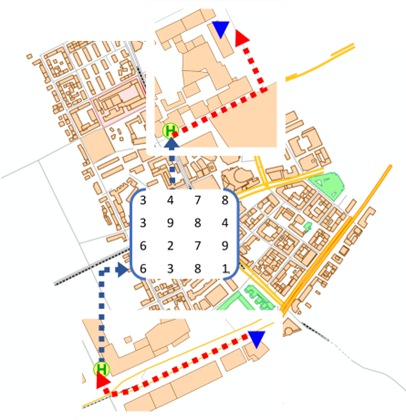
For public transport modes, a shortest path search other than the interactive shortest path search is used. The intermodal shortest path is composed of an inbound and outbound path to and from the stop area, respectively, and a matrix value of a stop area matrix. Access and egress paths are public transport walk paths, and an impedance matrix is chosen as the stop area matrix.

All stop areas that can be reached within a certain time can be considered as the start or end of the public transport path. The shortest path is then the path with the least impedance among all combinations of stop areas under consideration.
There is a reason for this particular type of shortest path search for public transport: the alternative direct use of the public transport timetable would require implementing a model for shifting the start time with respect to the timetable. Without such a model, the public transport mode might not be chosen only because the targeted bus would have departed on schedule a few minutes before the desired departure time. This would significantly increase the complexity of the demand model.
Such accuracy is not necessary. Although all start and travel times are calculated to the second, this does not mean that the demand model actually operates at this level of accuracy. With skims for each time range, exactly the level of accuracy is mapped that is useful for a demand calculation. Furthermore, it is not at all desirable, especially for demand calculations for the distant future, for the model to be correspondingly sensitive to the (necessarily) second-by-second modeling of a public transport supply that is not yet fully known.

