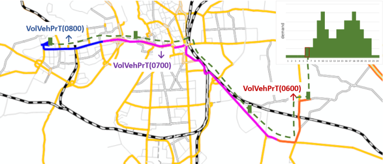
For each path in the assignment, demand is pushed along the path for each time interval. Here, demand originates from the demand time series and is assumed to be uniformly distributed within a time interval. It is advanced according to the travel times resulting from the assignment. The resulting dynamic volumes are stored in the volume attributes of the corresponding analysis time interval of the links, connectors, and (main) turns (see ). For the sake of simplicity, demand is already fully taken into account as soon as it enters a link, a connector, or a turn.
The supply of demand into the network begins at the start of the first analysis time interval. Therefore, if the time before the first analysis time interval is to be taken into account, a corresponding analysis time interval must be added. The supply of demand into the network begins at the start of the first analysis time interval. Therefore, if the time before the first analysis time interval is to be taken into account, a corresponding analysis time interval must be added.

Illustration 150: Exemplary representation of the distribution of demand from a time series to the analysis time intervals. The demand that starts at 6 o’clock reaches the first links in the time interval [6:00, 7:00] and the destination in the time interval [8:00, 9:00]. The volumes caused during the path are assigned to the corresponding analysis time intervals.
For very large models (> 1 million links) it may be useful to limit the number of threads (to, for example, 32), otherwise, the temporary memory requirements may become too high.

