Volumes always have at least an implicit time reference which they get from the time reference of the demand (if the demand matrix contains the demand of the peak traffic hour for example, the assignment results will also refer to the peak hour). To apply the resulting volumes to a shared time unit and then project them evenly to longer temporal horizons, the following analysis periods are provided in Visum.
- The calendar period covers the set calendar, i.e. one, seven or any number of days.
- The Time reference of the demand determines the number of travel demands within the assignment time period. The time reference is established by the start time of the demand segment and the time series allocated to the demand segment (User Manual: Managing demand objects).
- The Assignment time period mainly serves to determine the share of the demand that needs to be assigned. It is crucial that the assignment time period of each assignment lies within the analysis period. In the assignment, the share of the demand that accounts for the Assignment time period according to the time series is assigned to the paths found in this time period. The assignment area and the demand time series need to overlap, since otherwise no demand exists within this time period and no assignment can be calculated. An assignment time period can only be specified for dynamic assignments (Simulation-based dynamic assignment (SBA), DUE, Dynamic Stochastic assignment) of the PrT and for the headway-based and timetable-based assignment of the PuT. The assignment time period is specified in the parameters of the assignment procedure. In all statistic PrT assignments (LUCE, Bi-conjugate Frank-Wolfe, Equilibrium assignment, Incremental procedure, Equilibrium_Lohse, Stochastic assignment, Tribut), the assignment time period automatically corresponds to the analysis period.
- The Analysis period (AP) represents the period on which all evaluations are based. If no calendar is used, the analysis period is one day. When using a weekly or annual calendar, the analysis period can be specified, but must lie completely within the calendar period. The analysis period is a time period between at least one day and a maximum of the whole calendar period Initially, calculated results are available for the analysis period, before they are converted into analysis time intervals or the analysis horizon. The assignment time periods must lie completely within the analysis period. For the analysis period projection factors can be specified at the demand segments, which project the assignment results from the assignment time period to the analysis period. They serve to scale the demand to the analysis period. If the time period of the demand matrix is identical to the analysis period, the projection factor is 1. If the demand matrix is based on one day, yet the analysis period on a week, the factor would have to be set to 7 (when assuming that the traffic is the same on all 7 days of the week).
- The Analysis horizon (AH) is a longer time period over which results can be projected. It is not specified explicitly. Instead, the projection factors on the analysis horizon are predefined. These can be specified at the demand segment (for the volumes) and at the valid day (for the operator model) (Basic calculation principles for indicators). As a rule, an analysis horizon of a year is regarded. Since a different projection factor can be specified for each demand segment, the projection factor of daily values to a year can for example be smaller for a demand segment Pupils than for a demand segment Commuters, as the pupils have more vacation days on which they do not generate any traffic. The volume of a network object in terms of the analysis period is the total of the volumes of all paths traversing the network object, multiplied by the projection factor of the demand segment. This projection factor compensates that the assignment time period may cover only a part of the analysis period.
- Analysis time interval (AI)
For a more detailed time evaluation of calculation results, a time interval set can optionally be defined as the basis for analysis time intervals (Temporal distinction with analysis time intervals). Each analysis time interval needs to lie completely within a calendar day of the analysis period.
|
Note: Contrary to the analysis period, which incorporates the assignment time period and thus requires a projection of the volumes, the analysis time intervals identify the exact volume which arises in the respective time period. Thus, the projection factors of the individual demand segments do not have an effect on the volume per analysis time interval. If the analysis period is completely covered by analysis time intervals, the relationship between the total volumes for the intervals and the volume related to the analysis period exactly corresponds to the projection factor. |
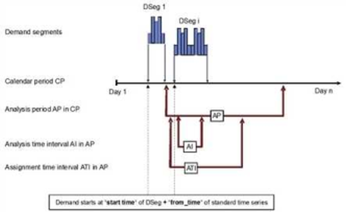
Image 37: The relationship between the different analysis periods
Example of projection factors
Volumes are to be determined per week in a model with a weekly calendar. To reduce the run time of an assignment procedure, the entire week should not be used as an assignment time period. It is assumed that the demand and the supply of week days Monday to Friday are the same. Demand data is available for the standard working day, Saturday and Sunday.
This is solved in the following way. Three demand segments are set, which each represent the demand on the working day, Saturday and Sunday. Each demand segment is provided with an appropriate time series, whereas the standard working day has to be one of the days Monday to Friday. Three assignments are calculated. The assignment time period is only one day, namely Tuesday (representing the standard working day), Saturday and Sunday.
A week is set for the analysis period and a year for the analysis horizon. The following projection factors are used, to correctly project the volumes.
|
Demand segment |
Projection factor AP |
Projection factor AH |
|
Standard working day |
5 |
|
|
Saturday |
1 |
52 |
|
Sunday |
1 |
52 |

Example of the interaction of analysis periods and time series
To calculate an assignment, the assignment time period and the time, which is valid for the demand, have to overlap. Three examples are shown below. In the first case (Image 38), the demand and assignment intervals do not match and the assignment cannot be calculated. Visum then issues the error message No OD pair shows demand > 0 within assignment time period. No connections calculated. In the second (Image 39) and third example (Image 40) assignment time period and validity period of the demand overlap so that an assignment can be calculated. The Table 13 provides an overview on analysis periods and time series of the three examples.
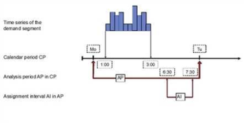
Image 38: Assignment is not possible as demand validity and assignment time period do not overlap.

Image 39: The demand between 6:30 and 7:30 a.m. is assigned.
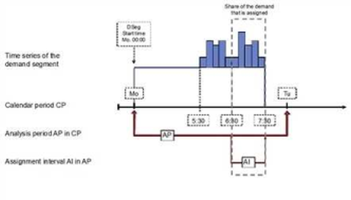
Image 40: The demand between 6:30 and 7:30 a.m. is assigned.
