Besides the direct attributes of the currently selected network object, you can also access its indirect attributes. These are direct objects of other network object types that are network model-related to the selected object. Therefore, for a network object, both the direct attributes as well as its relations to other network objects can be selected.
Indirect attributes give access to properties of other network objects, which bear a logical relation to the base object. It is often convenient to filter network objects not only by their own properties, but also by the properties of their logical neighbors in the network, or to display these properties next to their own properties in listings or graphics (for example displaying the aggregated values of the attributes of all stop points, which belong to a stop, in a list).
Relations between network object types are displayed explicitly in the user interface and allow access to all attributes of the referenced network object types (e.g. Link → From-node → Outgoing links). The three existing kinds of relations between the currently selected network object type and other network object types are indicated as follows.
-
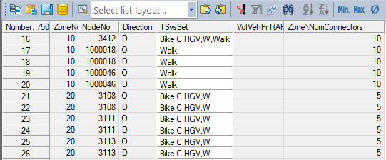
 exactly one relation (1...1). Such a relation, for example, exists between connector and zone: each connector connects exactly one zone with the connector node. In the example of Table 15, for connectors, the indirect attribute Zone\Number of connectors is output. For each connector, you can thus see how many other connectors the zone of this connector has.

-
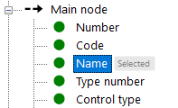
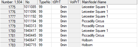
 either one or no relation (0..1). Such a relation, for example, exists between nodes and main nodes. A node can be allocated to a main node, but does not have to be. Besides, each node can be allocated to just one main node. As depicted in Table 16, with the aid of indirect attributes you can see for each node to which main node it is allocated by selecting the name of the main node as indirect attribute (Main node\Name).
-
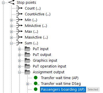
 several relations (0..n). Such a relation, for example, exists between stop areas and stop points. Since no 1:1 link exists between the network objects types in this case, you need to select an aggregation function which pools all related network objects (the aggregation function Sum for example ensures that all indirect attributes are allocated with the sum of, for example, all boarding passengers at all stop points that have a relation to the selected stop area). Below, an example is given for each of the aggregation functions provided in Visum.
If a 0..n relation has been selected at the Visum interface, the aggregation functions of either all network objects or merely the active ones are displayed. Aggregation functions are not provided in case of 1..1 and 0..1 relations, as there is only one relation from the current network object to another network object in this case (just one link type is for example allocated to each link). For 0..n relations, the following aggregation functions are provided:
- Count and CountActive
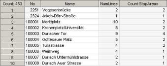
Determine the number of associated network objects. In Table 17, the number of stop areas associated with a stop is determined.

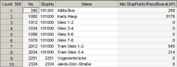
Determine the minimum value of all associated network objects for the selected attribute. In Table 18, the minimum number of boarding passengers at all stop points of the stop area is output.

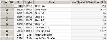
Determine the maximum value of all associated network objects for the selected attribute. The Table 19 displays the maximum number of boarding passengers at all stop points of the stop area.

- Sum and SumActive
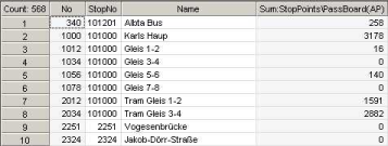
Determine the total of the values of all associated network objects for the selected attribute. The Table 20 displays the total of boarding passengers at all stop points of the stop area.
- Avg and AvgActive
Determine the mean of the values of all associated network objects for the selected attribute. The Table 21 displays the average number of boarding passengers at all stop points of the stop area.


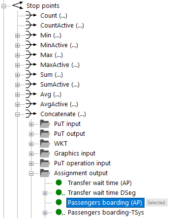
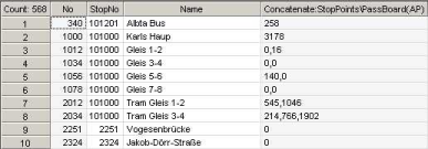
- Concatenate and ConcatenateActive
String all values of the associated network objects together for the selected attribute. The Table 22 displays the number of boarding passengers at each stop point of the stop area. At the stop points of stop area 2012 for example, 545 and 1046 passengers board each.
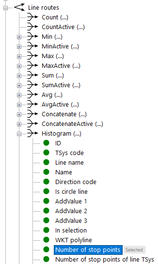
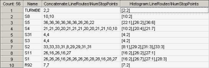
- Histogram and HistogramActive
Contrary to the aggregation function Concatenate, each occurring value is issued only once along with the frequency of its occurrence. This display offers more clarity especially if the user wants to see which values occur at all and how many times. The Table 23 illustrates the difference between the Concatenate and the Histogram display. Here, for each line, the number of stop points of the associated line routes is displayed. For example, 13 line routes are allocated to line S4. Two of the line routes have 10 stop points, 4 line routes have 20 stop points, and 7 line routes have 21 stop points.
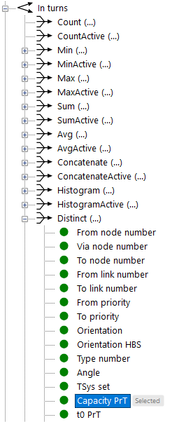
- Distinct and DistinctActive
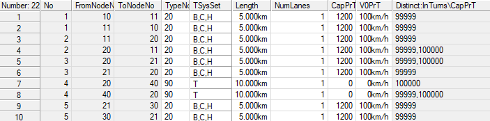
Contrary to the aggregation function Histogram, each occurring value is issued only once regardless of the frequency of its occurrence. This display offers more clarity especially if the user wants to see which values occur at all. Table 24 shows the difference between the Histogram display and the Distinct display. Here Capacity PrT of the entrance turns is displayed for each link.
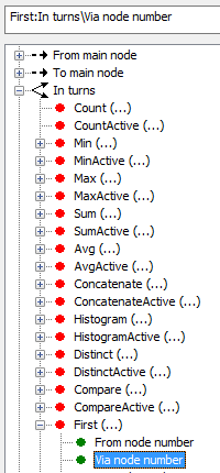
- First and FirstActive
Return the first or the first active element of a concatenation. Last and LastActive return the last value.
|
|
|
|
Selection of indirect attribute FirstValue:In turns\Via nodes_number in the Select attributes window |
The indirect attribute is displayed in the list next to the direct attributes of the link. |

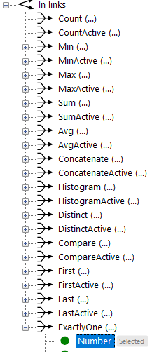
- ExactlyOne
Returns the value of an attribute if n=1 for a 1:n relation. In the example, the number of the link is output for the relation node to incoming link if there is only one incoming link.
|
|
|
|
Selection of the indirect attribute ExactlyOne:InLinks\Number in the attribute selection window |
The indirect attribute is displayed in the list next to the direct attributes of the node. |

|
Note: Indirect attributes can also be used as source attributes for operation Intersect and thus allow the combination of logical and geometric relations (Intersect). |
