The calculation of traffic flows for tour-based freight is performed in two related, successive procedures: In a first step, the procedure "Tour-based freight generation and distribution" is used to calculate order volumes and their spatial distribution. In a second step, the procedure "Tour-based freight trip generation" is used to calculate the actual trip matrices based on the orders.
Generation and distribution
The procedure Tour-based freight generation and distribution combines the steps of generation and spatial distribution of the orders. The procedure is closely based on the 4-step model(Standard 4-step model in two variants), but also has some particulars.
Generation
The productions of a demand stratum in a zone depend on its structural indicators that describe the intensity of the economic activity. Common indicators are the number of workplaces, factory space, number of cars or similar information. These indicators can mostly be derived from statistics and land use documents. In our case, they must be broken down by source sectors. In addition, production rates are required as a behavioral parameters that indicate how many orders are generated per structural skim unit. In general, the following formula is used to generate

orders:
During the procedure, the productions are calculated per demand stratum analogous to the 4-step model. The latter uses a production definition that can be freely defined by formulas. This allows you to flexibly derive skims from other values and maintain production rates in the data model. The productions determined are implicitly available in order units (not explicitly used in data model) and are saved to the attribute Productions(DStr) of the zones.
There are two alternative ways to calculate productions. Firstly, analogous to the 4-step model, productions can be defined by a formula. If productions and attractions have not already been evened out through the attributes and production rates used, you can set a procedure parameter to have them scaled to the same level. As reference values, you can predetermine total productions, total attractions or the minimum, maximum or mean value of both parameters.
In many cases it is difficult to determine the data and coefficients required for a direct calculation of productions, as surveys and statistics generally only provide data on the source (origin) sectors, but not on the target (destination) sectors. Alternatively, the attractions can be derived from the productions. In this case, additional information on economic interrelations is needed, i.e. data on how the total order volume of a source sector is distributed across the receiving sectors. This data can be obtained from company surveys. If such surveys are not available, you can fall back on publicly available statistics, such as the input-output accounts. In addition, the receiving potential of the receiving sectors in the zones must be described through indicators. Calculation of the attractions is then performed according to the following formula:
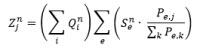
where
|
|
Productions at origin zone i for demand stratum n |
|
|
Attractions at destination zone j for demand stratum n |
|
|
Share of receiving sector e of total productions in demand stratum n |
|
|
Receiving potential of receiving sector e for destination zone j |
|
n |
Demand stratum |
|
e |
Receiving sector |
| i, j, k |
Zone indices |


In the procedure parameters, for each demand stratum, the program specifies its share in total productions across all receiving sectors and how the respective receiving potentials of zones in the receiving sectors are determined. The software also includes sectors that are merely defined as target (destination) sectors and are thus not directly assigned to a demand stratum, e.g. private households that are merely recipients of services. The attractions determined per demand stratum and receiving sector are then aggregated to the demand segments.
Both calculation options ignore possible external interrelations, i.e. it is always implicitly assumed that the total of order productions does not take place in the area examined and the receiving sectors are merely supplied by the area examined. In both cases, the results are saved per demand segment to the attribute Attractions(DSeg) of the zones.
You can limit calculation to the active zones. This might be useful in cases where the network model covers both the actual planning area and its surrounding sub network cordon zones. If you only want to calculate planning area-internal trips by means of the demand model, first of all define a filter for the zones of the planning area only. Proceed in a similar way if the production rates are not uniform for all zones. Break the zones down into groups of homogeneous production rates and insert the procedure Trip generation for each of the groups into the process. Prior to each such procedure, set a filter for the zones of that group (Procedure Read filter (Reading filters during a procedure sequence)) and calculate trip generation only for the respective active zones.
If the procedure is used in an iterative demand model that has a GoTo procedure(Iterative repetition), it might not make sense to have the generation recalculated with each iteration. This is why there is an option in the procedure parameters that only allows for generation calculation with the first iteration.
Distribution
Distribution entirely corresponds to trip distribution used in the 4-step model(Trip distribution). In lieu of OD trips, calculations are performed in the virtual unit order. Orders, however, do not explicitly occur. The result of the procedure is a distribution matrix of orders per demand stratum.
Trip generation
The procedure Trip generation is meant to create trip matrices from the distribution matrices for orders. As previously illustrated, with tour-based freight, several orders are supplied during the trip of a vehicle. The extent to which tours are created and the spatial characteristics of a tour vary depending on the sector and delivery concept used. The procedure Trip generation does not explicitly create tours as contiguous trip chains on a (microscopic) level of individual vehicles. Instead, the procedure uses a macroscopic approach and creates individual tour segments as trips between zones that are saved to joint matrices for all vehicles. For a (fictitious) tour of a vehicle belonging to a certain delivery concept of a certain sector, several types of trips are created:
- A start trip from origin zone to first order location (zone)
- If required, several connection trips between additional order locations are made
- A return trip from last order location back to origin zone
To determine spatial assignment of the different trip types, proceed as follows:
1. Determine start trips per origin zone
2. Spatial distribution of start trips
3. Determine outstanding orders and required connection trips
4. Spatial distribution of connection trips
5. Determine return trips
6. Output trip matrices
Determine start trips per origin zone
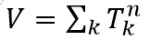
As the procedure uses a macroscopic approach, order assignment is not optimized (Traveling Salesman), but instead it is assumed that all tours of a demand stratum supply the same number of orders specified in the procedure parameters "Average number of orders per tour". All origin zone orders of a demand stratum (i.e. the row sums of the assigned distribution matrix) are distributed evenly across virtual tours. This results in the number of tours created in an origin zone kand thus in the number of start trips as

where
|
|
Number of tours of demand stratum n with origin zone k |
|
|
Productions of demand stratum n from origin zone k |
|
|
Average number of orders per tour for demand stratum n |


It can be assumed that the average number of trips per tour is greater than 1, i.e. that there are no empty trips.  is thus smaller than or equal to
  , which means there are normally orders left that are not supplied via start trips. These orders are supplied via connection trips between zones.
Spatial distribution of start trips
For spatial distribution of start trips, two aspects must be considered. Firstly, spatial distribution, as is common, follows a demand stratum-specific characteristic defined by skims (utility matrix) and a weighting function. Secondly, the attractions per zone determined through generation and distribution must be kept as an upper limit (boundary condition) - there must not be more start trips to a zone than the number of orders to be supplied. For this reason, a bilinear version of the multi-procedure is used, similar to EVA distribution and mode choice. With a soft, destination-sided constraint, fixing the total volume
 means
means
that the attraction total is also be fixed. Through this procedure, the start trips are distributed to the destination zones. This is done proportionally to the attractions as well as to the transformed utility of the destination zones, whilst the maximum value, the attraction in the destination zones, is observed. The results are listed in a matrix  .
.
Determine outstanding orders and required connection trips
The connection trips are considered separately per origin zone k. In a first step, it is determined which orders to be supplied from k to the destination zones are not covered via start trips. To do so, the start trips  are subtracted from the order matrix
  . The remaining orders
  must be supplied via connection trips between the destination zones.
Spatial distribution of connection trips
In this step, OD pairs are determined with which the required connection trips are realized. As for the spatial distribution of start trips, several aspects must be considered. The extent to which connection trips are optimized in terms of costs is different for the individual demand strata. Highly optimized sectors that generally handle the same type of mostly homogeneously distributed orders (e.g. parcel services) tend to realize large potential savings. In other sectors, where order processing is rather determined by factors such as fixed deadlines or the use of special resources and employees (e.g. service providers), cost optimization of the distribution trips plays a lesser role. Within the sectors, different optimization approaches for different logistics structures might be followed. Modeling of the OD trips thus depends on the cost matrices and a weighting function and varies between the demand strata.
As a boundary condition for determining connection trips, as previously for the distribution of start trips, the maximum attractions of the order distribution matrix must be observed. When skims are considered (e.g. run time), please note that due to the macroscopic approach, there is no information available on the sequence of order supply via connection trips. Instead of explicit trip chains, the distribution of connection trips is considered. It is thus not appropriate to use the skims (e.g. run time) for evaluation of the OD pairs between zones that are to be connected. Instead a procedure is applied that is based on the SAVINGS algorithm, which widely used for tour optimization. It is carried out with a reference to origin zone k:
For each pair in zones i and j (incl. k), the savings are determined that are obtained when two separate trips k- → i→ k + k→j→ k are replaced through a round tour with connection trip k→ i→ j→ k. In this case, the remaining attractions  must be > 0. Zone i could have also been reached with a start trip. Here the order volume must
  be > 0. The cost matrix used for the calculation
  corresponds to the utility matrix of start trip distribution.
As described further above, the extent to which potential savings are achieved is different depending on the demand stratum. For this reason, an evaluation of viable savings is performed with demand stratum-specific parameters. Note that here, unlike in the start trip distribution, savings are evaluated, not costs. Thus, while a monotonically decreasing function graph is used for the evaluation of the start trips, the graph for the weighting function of the savings is increasing. This means that if you use logit functions, for example, you should choose an opposite sign for the parameter c. If negative values occur when determining savings, then the transformed savings are mapped to zero. This happens independently of the weighting function used and should only occur if tours from k to i via j to k are more expensive than the sum of the tours k-i-k and k-j-k if the parameters are set correctly. In that case, the round tours are not used.
Then based on the evaluation results for the savings listed in a utility matrix, a bi-linear multi-procedure is calculated (see above). Thus the remaining orders  must be kept as a column total, i.e. as "hard", destination-sided constraints. For the row totals, the total number
  of orders is the upper threshold, as it is also the maximum number of connection trips that can start there. The
 are thus "soft", origin-sided constraints. The result is a matrix
  of all connection trips of tours that start in zone k.
Determine return trips
The return trips from zone i of tours that originated in zone k are determined as the difference between the total number of orders  delivered to i and the connection trips that start in i:

Output trip matrices
As a result of the calculation steps performed during the procedure, matrices are created per demand stratum for start trips, connection trips and return trips. These are then combined to total trip matrices per demand stratum. By default, the procedure only saves the total trip matrices. However, if required, you can also output other individual matrices. If applicable, the trip matrices may again be combined in the following procedure steps (Combining matrices and attribute vectors during the procedure sequence run), e.g. based on implicitly referenced transport systems or delivery structures. These aggregated matrices can then be assigned to the road network during an assignment procedure and be evaluated, e.g. in terms of emission levels.
