The rubber banding function was implemented to make the choice of destinations and modes along an activity chain more realistic. The idea behind it is that the destination choice for all activities is made based on a main activity, which allows us to determine more consistent route chains. Mode choice is based on the main activity and not on the first destination activity.
In the Combined distribution/mode choice, the destination choice for an activity transfer takes into account not only the location of the origin activity but also the home location or location of the main activity of the chain (e.g. workplace). The impedance is not considered in isolation from an activity, but as a total of impedances from the home location via an in-between activity to the main activity. A scaling parameter w needs to be defined which determines how the path legs’ impedances between the in-between activity and the main activity are weighted against each other.
The main activity can be defined by specifying the rank. The rank is an activity attribute. The smaller the number, the higher the rank (and the more important the activity). The main activity is the top-ranking activity within the activity chain. If there are multiple top-ranking activities, the first activity is rated as the main activity.
Rubber banding only shows effect if the activity chain outside the home location consists of at least two activities. The activity chain home-work-home (HWH) is not calculated any differently when you include the rubber band function. Important is how you define the main activity. It determines where the weighting is carried out.
An example calculation:
In our example, the activity chain consists of the activities home-shopping-work-home (HSWH). Our main activity shall be work.

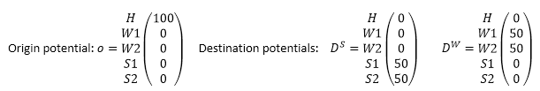
The above figure depicts the position of the activity type as well as the impedances between the activities. The origin demand is 100 persons. There is a destination potential for the workplace and shopping of 50 persons each.
Thus the following applies:
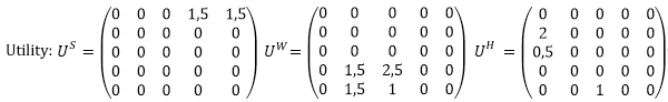
To calculate the destination choice, we will use a Logit function, with c = 1, i.e. f(u)= e-u. Without accounting for rubber banding in our calculation, only activity transfer H-S will be considered for the destination choice. As the utility of S1 and S2 are the same when starting out from the home location, namely 1.5, 50 persons each choose S1 and S2 in the calculation scenario without rubber banding. This scenario, however, does not account for the fact that for persons working in W2 it is more convenient to shop in S2, as the utility (impedance) from S2 to W2 is 1, whereas the utility from S1 to W2 is 2.5.
In the rubber banding calculation scenario, the destination choice for the main activity is calculated first. This is also the case when, as in the example, the main activity is not the first activity, and there is no direct transfer of activity from H to W. The same applies to mode choice, which is based on the activity transfer from home activity to main activity.
Step 1: Destination choice H->W


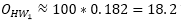
The number of trips from home to work is thus
 and
and 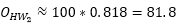
These, however, include several legs: Part of the legs traverses S1, whereas the other part traverses S2. As there is no data available on individual legs yet, and we merely distributed the origin potential of 100 persons across the zones for the main activity work, we will call the new matrix OH→W, or destination-related origin potential.
The exact distribution across individual paths, i.e. which town the persons choose to shop in depending on their workplace is calculated in the next step.
Step 2: Destination choice H->S
As the shopping location is chosen depending on the destination choice for the main activity, the shopping location choice is determined separately for the workplaces W1 and W2. Utility  is replaced with
  . The factor w determines the impact of the rubber band, i.e. the effect between the in-between activity and the main activity. In our example, w = 1 the weighting between both path legs is the same.
This means, for persons working in W1 the following applies:

Persons working in W1 are equally likely to shop in S1 or S2.
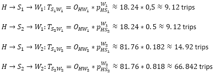
Accordingly, persons who work in W2:

As S2 is much closer to W2 than S1, more people working in W2 go to S2 to shop.
Now we can calculate the trips from home to S1 and S2.


Step 3: Destination choice S->W
We determined the destination choice for the activity work in Step 1. Now we only need to expand the leg combinations.
If there are several home locations, the legs must also be added.
Step 4: Destination choice W->H
As everyone returns to their home location, a destination choice is not determined in this case. Our path matrix is simply a transpose matrix SH→W of Step 1, namely

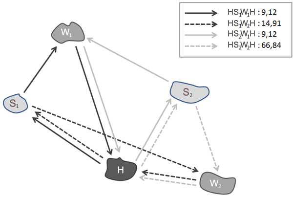
The activity chains and volumes are depicted in the following figure.
Cases with more activity chains than shown in the above example require special steps. It is then Important how you define the main activity.
1. If you extend the activity chain in our example by activity B (for bakery) to HBSWH, during calculation of legs FH→B, the activity shopping is initially ignored. The relevant activity chain is then HBW. First, as in our example, the destination-related production SH→W and the path matrix FH→B are calculated. By adding the trips in the next step, we determine a destination-related production starting at activity B, with OB→W. Afterwards we can look at the remaining chain up until the main activity, namely BSW. We calculate the destination choice B→S as in Step 2: For each destination zone k of the main activity W, we replace the utility with S (for the destination choice), that means  with
with  .
.
2. If between the main activity and home there is another activity (e.g. HWSH), our calculation between W and H is based on a total impedance between W and H. For a fixed destination zone k for H, you then replace with  for the destination choice S.
The scale parameter w determines the weighting of the impedances of the path legs between the in-between activity and the main activity in contrast to the other path leg. A value of w = 1 means that both path legs are weighted equally. A value range of 0,5 ≤ w ≤ 2is recommended. A 0 value indicates a calculation without rubber banding. By selecting a very high value for w a proportionally high weighting would be given to the second path leg. The destination choice for the in-between activity would then be very close to the main activity.
