Construction of the graph

These are the basic steps for constructing the graph:

1.  For each departure and arrival of a vehicle journey section (or a sequence of vehicle journey sections connected by forced chainings) insert a node and connect both nodes with an edge. Below, these nodes are called 'real events'. Departure and arrival in each case is the time including possible pre- and post-preparation times if these are taken into consideration (User Manual: Parameters of the line blocking procedure).

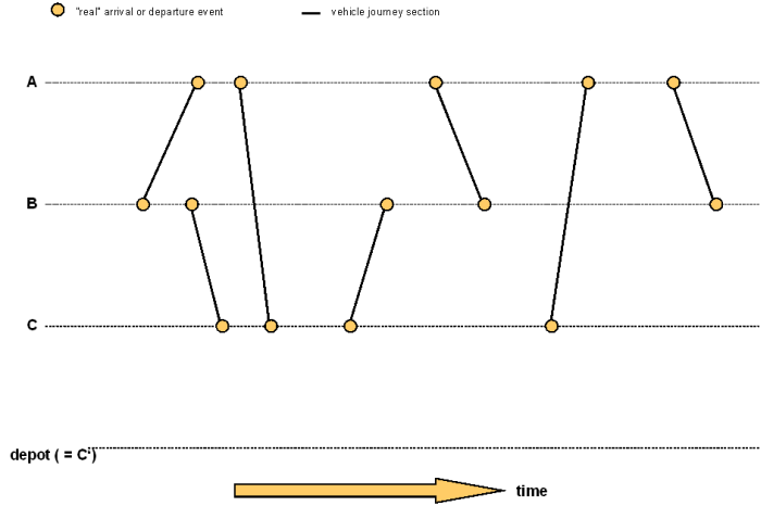
Image 190: Inserting the nodes and edges for vehicle journey sections

2.  For each permissible depot for the vehicle combination as well as for each stop point, which is the start of a vehicle journey section of the current partition (empty trips between stop points), enter an arrival event for the time of arrival and an edge for the empty trip from the departure event of the trip to the arrival event at the stop point or depot (so-called unreal or "fake" arrival events are thus created). Depots are thus special stop points. In the graph, the events at stop points and in depots are distinguished – which means, that in the graph there is one node for the stop point and another one for the depot, although the depot is represented by the same stop point in the network.

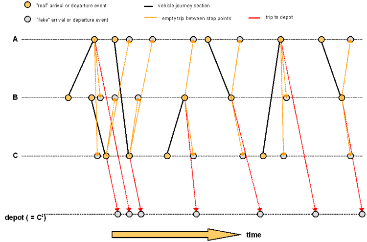
Image 191: Inserting the edges for entering the depots and for empty trips between stop points

3.  Analogously, insert also a departure event and an edge from there to the departure event of the trip, however, only for each permissible depot, not for other stop points (these mean moving out of the depots, so-called fake departure events are created in this way).

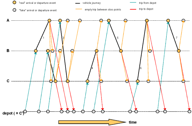
Image 192: Inserting the edges for leaving from depots

Note: If interlining is prohibited (User Manual: Parameters of the line blocking procedure), only edges from and to that depot are inserted, which is represented by the same stop point in the network. Thus, interlining is not possible in this case, the vehicle combination can however, enter a depot and subsequently return to the same stop point for the start of the next trip.

4.  Insert an additional edge (the so-called Timeline or Waiting edge) between each pair of succeeding events of a stop point or depot. Using this edge, it is possible to model waiting (downtimes) at a stop point or in a depot. Timeline edges thus make it possible, that a block can be continued with a new trip at the same stop point.

For line blocking you can select whether you want to create open or closed blocks. With the generation of closed blocks, each timeline, therefore each sequence of timeline edges for a stop point or a depot, generates a closed ring. Vehicle journey edges and empty trip edges can also cross the transition from the last to the first day of the blocking time interval. A block has as many blocking days as it makes "rounds" through the calendar period, until it has reached its starting point again.

Only for open line blocking it can be claimed, that blocks start and end in depots. Connecting edges are then inserted before the first node and after the last node of a timeline, from an auxiliary node to all depots. Inflow and outflow only takes place via this auxiliary node. In this case it may occur, that no flow can be determined. This happens when the total capacity of all depots is smaller than the number of vehicles required to cover all actions. In such a case, line blocking is canceled with an error message.

Also in the introductory example (Open and closed blocks) you can find a note concerning open and closed line blocks.

5.  The graph is now simplified, by combining nodes with the same accessibility and by deleting equivalent empty trip edges (which provide access to the same departure). The graph after the edge reduction can be seen in Image 193.

Image 193: Example graph after inserting the timeline edges and edge reduction

6.  For the formulation as a flow problem, it is necessary to define a lower capacity limit and an upper capacity limit to the edges (which is the number of vehicles which can maximally or minimally flow via an edge). The following applies:

• The lower limit of the capacity on the vehicle journey sections is 1 (because it is mandatory that each vehicle journey section is really traversed).
• All other edges have a lower capacity limit of 0 (because traversing is not mandatory, for example for empty trips).
• The upper limit for the vehicle journey section edges is also 1 (because each vehicle journey section should only be traversed exactly no more than once).
• Empty trip edges as an upper limit have the number of empty trips, which they represent (this is only greater than 1 if, in the framework of edge reduction, edges were combined).
• Edges along the timelines, if a depot, use the depot capacity as upper limit. For all other timelines the upper limit is not restricted.

7.  To be able to determine a cost-efficient flow, the edges with costs have to be evaluated in the last step. These are described by a cost function analog to the perceived journey time for PuT assignments (Perceived journey time). This cost function is made up of summands, which each multiply one property of the edge (therefore the activity described by the edges) by a factor and a cost rate. The cost function is as follows:

Cost	= Required vehicles • Coefficient • Cost rate vehicle unit total
	+ Service time • Coefficient • Cost rate hour service
	+ ServiceKm/Mi • Coefficient • Cost rate Km/Mi service
	+ Space • Coefficient • Cost rate hour empty
	+ EmptyKm/Mi • Coefficient • Cost rate Km/Mi empty
	+ Number of empty trips • Coefficient
	+ Layover • Coefficient • Cost rate hour layover
	+ Service time depot • Coefficient • Cost rate hour depot
	+Charge time • Coefficient • Cost rate hour charging

Note: The coefficients also have an effect on the cost rate for "no vehicle combination".

Which cost components have an effect on an edge, depends on the edge type. The cost components for the individual edge types are the following.

• Vehicle journey edges
• Service time describes the duration of the vehicle journey section (The costs for the trip itself are irrelevant for solving the problem, because each edge is allocated with exactly one flow of 1 and there is thus no alternative allocation. To display the result, vehicle journey edges are still evaluated with the vehicle journey cost rates of the vehicle combination for duration and distance.)
• ServiceKm/Mi describes the distance covered by the vehicle journey
• Layover describes the duration between the From-node's point in time and the departure from the From-node plus the duration between the arrival at the To-node and To-node's point in time.
• Empty trip edges
• Empty time describes the duration of the empty trip
• EmptyKm/Mi describes the distance covered by the empty trip
• Layover describes the duration between the From-node's point in time and the departure from the From-node plus the duration between the arrival at the To-node and the To-node's point in time, in case it is a normal stop point
• Depot layover describes the duration between the From-node's point in time and the departure from the From-node plus the duration between the arrival at the To-node and the To-node's point in time, in case it is a depot
• Timeline edges
• Layover and layover depot describe the length of the time period between the points in time of the nodes which are connected via the edge
• To evaluate the vehicle demand, for each edge which traverses a selected point in time, the cost rate for the vehicle combination is added to the evaluation. Because each vehicle combination has to traverse this evaluation point in time exactly once, the vehicle demand is thus counted and evaluated.

As an interim result, an evaluated graph is available, for which a flow with minimum costs is determined in the following step.