For projection to the analysis horizon, the indicators of transport demand (network performance, revenues), the indicators of the transport supply (operating supply, costs), and the hourly costs are each projected with a different factor. This takes the fact into account that the transport demand, for example at the weekend, can decline more severely than the transport supply. At the same time, there are higher personnel costs, i.e. higher hourly cost rates on Sundays.
The projection factors for transport supply and hourly costs can be specified for each valid day separately. In this way, for an analysis period of one week in August, not only can the indicators of regularly occurring Valid Days be correctly projected to an analysis horizon of one year (for example, Mon-Fri with factor 52), but also seasonally restricted Valid Days (for example, Sat+Sun during the school summer holidays by applying factor 6).
The projection factors for the extrapolation of the network performance from the assignment time period to the analysis period or horizon are set separately for each demand segment. Therefore, the projection factor from the assignment time period to the analysis period regards the relevance of the OD matrix content for the demand segment.
- If the assignment time period and the period of validity of the matrix cover the entire analysis period, this factor is then equal to 1.
- If the assignment time period is shorter than the analysis period, then the projection factor corresponds to the ratio between the demand in the analysis period and the demand in the assignment time period.
- If the demand time series of the demand segment refers to only a part of the assignment time period, then the projection factor corresponds to the ratio between the demand in the analysis period and that of the demand time series time period.
The following example shows how this kind of calculation can be used to save computation time in case of homogeneous demand.
Example
The analysis period and the assignment time period should each cover one week (Monday to Sunday). The timetable services from Monday to Friday are identical. For the "commuters" demand segment the demand from Monday to Friday may be constant and the same time series may be applied on weekdays, whereas on the weekend there is no demand in this segment. The demand of this demand segment is coded in the OD matrix of one day in combination with the time series for 24h, beginning Monday at 0:00. Due to the time series, only the trips which start on Monday are charged during assignment. In order nevertheless to indicate correct weekly values as PuT volumes per analysis period, the following projection factors are applied to the "commuters" demand segment.
|
Projection from ... to ... |
Factor |
|
Assignment time period→ AP |
5 |
|
Assignment time period → AH (= year) |
5 • 52 = 260 |
The following example of a vehicle journey with two sections (Image 208) shows the calculation of selected operating indicators for the following analysis times.
- the analysis period of one week
- the analysis horizon of one year
- an analysis time interval on Tuesday 7 – 8 a.m.
As shown in Image 208 and Table 266, vehicle journey section 1 is served daily, whereas vehicle journey section 2 is available on Sundays and public holidays only.
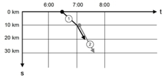
Image 208: Time-distance diagram for a vehicle journey with two vehicle journey sections
|
|
VehJourney |
VehJournSect 1 |
VehJournSect 2 |
|
Valid day |
|
Daily |
Sunday+Holiday |
|
Projection factor Analysis Horizon |
|
52 |
63 |
|
Departure |
6:30 AM |
|
|
|
Arrival |
7:30 AM |
|
|
|
Trip length |
30 km |
30 km |
|
|
Trip length 6:30 - 7:00 AM |
10 km |
10 km |
|
|
Trip length 7:00 AM - 7:15 AM |
10 km |
10 km |
|
|
Trip length 7:15 AM - 7:30 AM |
10 km |
||
|
Seat capacity |
|
200 |
100 |
Table 266: Further specifications for the vehicle journey with two VJ sections
The Table 267 shows the calculation of the seat kilometers. This is done by multiplying the seating capacity by the service trip length and then simply adding up the vehicle journey section data.
|
Analysis period Mon-Sun |
|
|
VehJournSect 1 |
200 seats • 20 km • 7 days = 28000 km |
|
VehJournSect 2 |
100 seats • 20 km • 1 day = 2000 km |
|
Sum |
30000 km |
|
Analysis horizon |
|
|
VehJournSect 1 |
28000 km • 52 = 1456000 km |
|
VehJournSect 2 |
2000 km • 63 = 126000 km |
|
Sum |
|
|
Analysis time interval Tue 7:00 – 8:00 |
|
|
VehJournSect 1 |
200 seats • 10 km = 2000 km |
|
VehJournSect 2 |
100 seats • 0 km = 0 km |
|
Sum |
2000 km |
Compared to seat kilometers, the calculation of service kilometers (often termed load kilometers or train kilometers) by simply adding up the vehicle journey sections is not permitted. In this case, it must be realized that superimposed vehicle journey sections may only be counted once. This is particularly important for the calculation of any track costs derived from the service kilometers. Track costs are calculated on the basis of service kilometers regardless of the train composition. In the projection to the analysis horizon, however, different projection factors may arise for the vehicle journey sections. In this case a maximum formation is taking place. In the example shown in Table 268, this is the case on Sunday. The calculation of the service time is carried out in the same way.
|
|
Analysis period Mon-Sun |
Analysis horizon |
Analysis period Tue 7:00-8:00 |
|
Monday |
20 km • 1 |
20 km • 52 |
10 km • 0 |
|
Tuesday |
20 km • 1 |
20 km • 52 |
10 km • 1 |
|
Wednesday |
20 km • 1 |
20 km • 52 |
10 km • 0 |
|
Thursday |
20 km • 1 |
20 km • 52 |
10 km • 0 |
|
Friday |
20 km • 1 |
20 km • 52 |
10 km • 0 |
|
Saturday |
20 km • 1 |
20 km • 52 |
10 km • 0 |
|
Sunday |
10 km • 1 + 10 km • 1 + 10 km • 1 |
10 km • 52 + 10 km • MAX 52;63) + 10 km • 63 |
20 km • 0 |
|
Sum |
150 km |
8,020 km |
10 km |
