For each origin zone, a search tree of suitable partial connections is generated which stores all sufficiently suitable connections from this origin zone. This means that not only the best connection is found for an OD pair, but a large number of good connections. In this way, a very selective distribution of travel demand is possible.
- A search impedance is used in order to evaluate the quality of connections. For all (partial) connections found in the search, the search impedance is calculated using the following equation:
SearchImp = In-vehicle time • FacIVT +
PuT-Aux ride time• FacPuTAuxRT +
Access time • FacAccT +
Egress time • FacEgrT +
Walk time • FacWlkT +
Transfer wait time • FacTrWaitT +
NRT • FacNRT +
Transport system impedance • FacTSysImp +
Vehicle journey impedance • FacVJImp
- For the in-vehicle time or PuT-Aux, additional specific factors of attributes from vehicle journey sections or transport systems may be used.
- Besides various time components and the number of transfers, these include TSys-specific supplements listed under Transport system impedance. That is, how common distance-based fares can already be considered during the search. The complete Visum fare model will take effect during the connection choice. However, this is no restriction, since the approximate fare calculation during the search is sufficient for the distinction between reasonable routes and useless ones.
- In addition, via Vehicle journey impedance, the vehicle journey-specific impedance is added. It results from two freely selectable attributes of the vehicle journey items – as boarding supplement and as general discomfort term. In this way, individual vehicle journeys can be favored or penalized.
- (Partial) connections to a destination or intermediate node are evaluated and compared with any other (partial) connection to the same point. Then it can efficiently be decided which branches of the search tree can be continued ("branch") and which have to be cut ("bound") (Dominance and Bounding).
- It is possible to specify an upper limit for the number of transfers in a connection.
Dominance
Pairwise comparisons are helpful for the identification of useless connections.
If a connection is in no respect more appropriate than another connection in the same temporal position, then this connection is called dominated and will be discarded. This means in detail:
A connection c’ dominates a connection c if
- c’ lies within the time interval of c
- NumTransfers (c’) ≤ NumTransfers (c)
- SearchImp (c’) ≤ SearchImp (c)
- and if
- real inequality applies to at least one of the three criteria or
- both connections are equivalent (Equivalent connections)
To compare two connections without defined temporal position (that means: without path legs of the 'PuT line' type) the first rule is changed to the following: Journey time (c’) ≤ journey time (c).
When evaluating partial connections, it may be useful to consider the wait time until the arrival of an alternative partial connection.
Path legs without a defined temporal position (e.g. pure DRT path legs) cannot be dominated by path legs with a defined temporal position.
Example:
- Connection 1 dominates connection 2, since it is really located in the time interval of connection 2 and because other indicators of connection 1 are either as good as those of connection 2 or even better.
- Connection 1 does not dominate connection 3, since the temporal positions differ, nevertheless connection 1 might be useful for those passengers who want to depart later though the indicators of connection 1 are worse.
- Connection 1 does neither dominate connection 4, since connection 4 does not require as many transfers as connection 1 which might be acceptable for some passengers though this means a longer journey time.
- (Partial) connection 1 does not dominate (partial) connection 2 if the wait time up to 7:10 is taken into account by the corresponding option, since passengers use a continuing connection at a time past 7:10, for example
|
Criterion |
Connection 1 |
Connection 2 |
Connection 3 |
Connection 4 |
|
Temporal position |
6:00 - 7:00 a.m. |
6:00 - 7:10 a.m. |
6:10 - 7:20 a.m. |
5:30 - 7:20 a.m. |
|
Number of transfers |
1 |
1 |
2 |
0 |
|
SearchImp |
4000 |
4200 |
4300 |
5400 |
Equivalent connections
Equivalent connections represent a special case regarding dominance. Two connections are considered equivalent when they merely differ in the selection of transfer stops, but are the same in terms of departure time and sequence of the time profiles used.
If the connections have path legs without a temporal position (DRT, Sharing, PuT Aux), the definition of equivalence is adjusted slightly: all path legs without a temporal position are then treated as a single time profile. In addition, a coinciding temporal position is given if the first and the last part of the path leg, which is made with a regular public transport line, use the same vehicle journey. In particular, this is equivalent to connections of the type "DRT –> public transport line", which board the same vehicle journey at different stops.
If the dominance of equivalent connections is allowed, the connection with the highest priority (smallest numerical value) dominates all connections with lower priority from a bundle of equivalent connections. If the priorities are the same, you define whether the connection should remain with the earliest or latest possible transfer. The transfer priority can be set at stop areas and between two vehicle journeys (planned connecting journeys). The priorities of the levels are added up. The connection with the highest priority (smallest numerical value) remains as connection. A default priority of 8 applies to stop areas and planned connecting journeys. It is assigned to all elements that are not defined.
If equivalent connections are allowed, a larger amount of nearly identical connections can be created. Please note that the choice model cannot account for the hierarchies within a set of connections. In some cases, using the independence factor allows you to compensate for this fact.
|
Note: Deactivating the independence factor while using equivalent connections can lead to unrealistic results. We therefore strongly recommend that you select the Use independence option when allowing equivalent connections. |
Example
Let us look at the network depicted in Image 159.
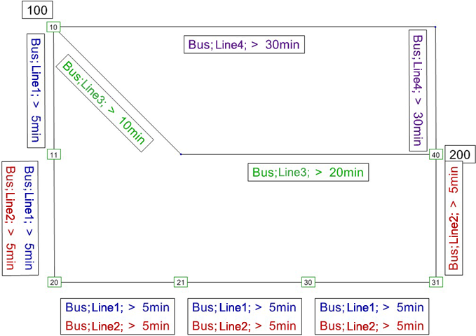
Image 159: Example equivalent connections
When we use lines 1 and 2, the following equivalent connections are created:
| Connection | From-Time profile | To-Time profile | Transfer stop point |
|---|---|---|---|
|
A1 |
Bus, line 1 >, 1 |
Bus, line 2 >, 1 |
11 |
|
A2 |
Bus, line 1 >, 1 |
Bus, line 2 >, 1 |
20 |
|
A3 |
Bus, line 1 >, 1 |
Bus, line 2 >, 1 |
21 |
|
A4 |
Bus, line 1 >, 1 |
Bus, line 2 >, 1 |
30 |
|
A5 |
Bus, line 1 >, 1 |
Bus, line 2 >, 1 |
31 |
If dominance is allowed with equivalent connections, only connection A1 remains available.
Example with independence
| Connection | Path leg(s) |
|---|---|
|
A |
Departure 6:30 with line 1 Transfer to line 2 in overlapping area of stop events 11, 20, 21, 30 and 31, TWT = 0 Arrival 7:00 |
|
B |
Departure 6:35 AM with line 3 Arrival 7:05 AM |
|
C |
Departure 7:00 AM with line 4 Arrival 7:30 AM |
Without independence factor:
When not using equivalent connections, each of the three connections is assigned a 1/3 share if the impedance parameters are set without a penalty for transfers.
If equivalent connections are allowed, connection A (with transfer at stop event 11) forms the basis for 4 additional options (A2 to A5) that only differ in terms of their transfer point. The set of connections now consists of seven equally good connections, and if the independence factor is not applied, each connection is assigned 1/7 of the demand. This case shows that when the independence factor is not applied, the choice model produces unrealistic results.
With independence factor:
When the independence factor is used in our initial situation, the demand is shifted towards connection C, as the temporal positions of A1 and B are very similar. C is now assigned 47%. The remaining demand is divided between the other two connections.
If equivalent connections are allowed, the share of C hardly changes. However, a large part of the demand shifts from B to A, as A1 to A5 do not only influence each other, but also reduce the independence of B. This case shows that when using the independence factor, you obtain better results. However, it also demonstrates the limits of independence.
|
Independence factor deactivated |
Independence factor activated |
||
|---|---|---|---|
|
Equivalent connections |
Equivalent connections |
||
|
No |
Yes |
No |
Yes |
|
33.3 % |
71.4 % |
26.5 % |
41.8 % |
|
33.3 % |
14.3 % |
26.5 % |
10 % |
|
33.3 % |
14.3 % |
47 % |
48.2 % |
Bounding
Besides the temporal position, the following rules are applied to exclude connections which differ considerably from the optimum in one or several criteria:
A (partial) connection is deleted if
- Search impedance of the connection > minimum search impedance • factor + constant, or
- Journey time of the connection > minimum journey time • factor + constant, or
- Number of transfers of the connection > minimum number of transfers + constant.
As a matter of principle, connections which are optimal in one of the three dimensions will not be deleted in this step, even if they violated the rule of another dimension.
