Assignment analysis is used for calculating the correlation (Goodness-of-Fit Report) between calculated and observed attribute values of a selected network object type.
- The calculated value is derived from the assignment or the network model.
- The observed value may be count data or measured data.
Here are some examples:
- Travel time comparisons between PrT and PuT
- Travel time comparisons of different scenarios
- Calculated and counted volumes (links, turns or main turns)
- Calculated and measured speeds
Any numeric input and output attributes of the following network objects can be selected:
- Links
- Node
- Turn
- Main nodes
- Main turns
- Lines
- Line routes
- Screenlines
- Time profiles
- Paths
Prerequisite is, that the observed values must be >0 for the selected network object type.
You can select which objects you want to include in the assignment analysis. There are three possibilities:
- All objects of the selected network object type
- Only active objects
- Only objects with observed value > 0
For the assignment analysis, as an option, you can consider user-defined tolerances for user-defined value ranges of the calculated attribute.
The quality of the correlation can be determined and issued in two ways:
- in groups (for each value of the classification attribute)
- collectively for all included network objects
For the output, the data model of the network object types above has been supplemented with the calculated attribute Assignment deviation (AssignDev) of type real. Alike all other Visum attributes, the attribute can be graphically displayed and issued in lists of the respective network object.
In addition, Visum calculates various indicators (per group or collectively) that can be issued in a list or in a chart.
|
Note: An assignment result is no longer necessary in order to calculate the correlation coefficient. |
The Table 194 shows the calculation rules for the output attributes of the assignment analysis. In the formulas, the following applies:
|
Z |
Observed value (counts or measures) |
|
U |
Calculated value (assignment or network model) |
|
N |
Number of objects with observed value > 0 |
|
AbsRMSE Abs RMSE |
Absolute root of mean square deviation Significant differences between counted and modeled values have a higher impact according to
|
|
Intercept Intercept |
Coefficient b in linear regression Cf. Excel, linear regression (y = ax + b) |
|
ShareAccGEH Share with acceptable GEH |
Percentage objects with acceptable GEH value (per network object)
|
|
ShareAccRelErr Share with acceptable relative errors |
Percentage objects within tolerance
|
|
NumObs Number of observations |
Number of observations per class (objects with observed value > 0) |
|
NumClass Number in class |
Total number (=observed + not observed) objects per class |
|
ClassVal |
Value of classification attribute (or blank if not classified) |
|
Corr |
Correlation coefficient (cf. Excel function Pearson) Notes The value range lies between -1 and 1, where the following applies:
The observed/modeled value ratio should be as close to 1 as possible. If only 2 values > 0 are used, the correlation coefficient is -1 or 1. From the value of the correlation coefficient, one cannot determine whether all observed values are higher (or lower) than the calculated values or upward and downward deviations exist. |
|
AvgAbsErr |
Mean absolute error Mean deviation of absolute values (δa) (Difference between observed and modeled value)
|
|
AvgObs |
Mean observed value |
|
AvgRelErr |
Mean relative error Mean deviation of absolute values in % (δp) according to
|
|
R2 |
Coefficient of determination r2 Cf. Excel function RSQ |
|
RelRMSE |
Relative root of mean square deviation
|
|
StdDev |
Standard deviation |
|
Slope |
Coefficient a in linear regression Cf. Excel, linear regression (y = ax + b) |


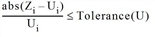


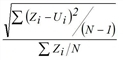
Table 194: Calculation rules for the output attributes of assignment analysis
