All distribution models presented (Distribution models in the assignment) cannot, in their basic form, take into account interactions between different connections in a timetable-based assignment. However, ignoring this aspect can be a drawback.
In order to model interactions, one defines functions wi, which describe the impact of other connections on a connection i. The value range of wi is the interval [0.1]. If j has no impact on i, then wi(j) = 0. If i and j are absolutely equal, then wi(j) = 1, meaning it is always wi(i) = 1.
The following values are used to calculate wi(j).
- The temporal proximity of the connections with regard to departure and arrival
- The advantage of i over j in terms of the perceived journey time
yi(j) := PJTj - PJTi
- The advantage of i over j in terms of the fare
zi(j) := Farej - Farei
Thus, wi is defined as follows:
 ,
,
where 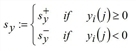 and
and 
The s > 0 are internal parameters for controlling the ranges of influence of the three variables. c is a constant which controls the absolute effect of the second factor and is given by the user within [0,1].
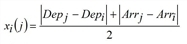
The first value describes the temporal proximity of i and j. If the times are the same, then xi(j) = 0, so that this value is equals to 1. If the time difference is xi(j) ≥ sx, the value becomes zero and wi(j) = 0 also applies. Thus, sx is the maximum temporal distance in which j can effect i.
If at least one connection has no temporal position (e.g. DRT paths), the first factor cannot be determined in the way described above. It is then defined as follows:
- 0 if exactly one connection has no temporal position
- 1 if both connections have no temporal position
The second value lies between 1 (in case of absolute equality in the context of yi(j) = 0 and zi(j) = 0) and 1 - c (when there is a significant difference between i and j). As with sx, sy+ or sy- is the maximum temporal advantage or disadvantage of i, in which j can possibly have an impact. With regard to the fare, the same applies to sz. The default setting leads to the following relation of sy- = 2sy+ and sz- = 2sz+. As a result of this asymmetry, in the case of two connections with temporal proximity, the better is favored, because its influence on the worse alternative is greater than vice versa. In principle, users should always specify Independency coefficients for high or low quality in the form of IndCoeffQualityHigh (ECQH) < IndCoeffQualityLow (ECQL). When violating this rule, a warning appears at the start of the assignment (or an error message in the window).
Overall, the following applies:
sx = min (2 • mean wait time of a random passenger between the first and the last departure, maximum time slot)
sy+ = ECQH • mean PJT in the total assignment period
sy- = ECQG • mean PJT in the total assignment period
sz+ = ECQH • mean fare in the total assignment period
sz- = ECQL • mean fare in the total assignment period
|
Note: Only the temporal positions, the PJT values and the fares are compared; service trip item data is not evaluated. |
If no fares are available (i.e. FPi = 0 for all i), then sz = 1 is set.
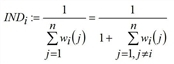
The attribute independence of a connection is now defined as follows:
 o
o
Here, n is the total number of connections.
Distribution models with independence
If independence is used for connection choice, then this attribute must be integrated in the distribution model. In the version described above, for each time interval a the utility Uia of a connection i was calculated. From this, its percentage in terms of the demand was determined per time interval. If independence is applied, Uia • INDi replaces Uia, i.e. the following applies:
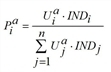
This linear dependence on the independence attribute ensures that k simultaneous, identical alternatives are treated as a single connection. According to the definition of IND, the independence of each of such k alternatives is precisely 1 / k (if no other connections with temporal proximity have an effect). As a result, the total of its weights in the distribution formula is equal to the weight of a single, non-multiplied connection of the same kind.
Comparison of the choice models with independence
In Table 185 to Table 189 the different choice models are compared with each other, with and without independence. The procedure parameters are chosen as in Table 184.
Connection data that differs from the respective previous example is highlighted bold in Table 189 to Tabelle 171. All assignment shares are given as percentages.
|
Connection data |
Distribution without IND |
Distribution with IND |
||||||||||
|
No. |
Dep |
Arr |
PJT |
Fare |
Kirchhoff |
Logit |
Box-Cox |
Lohse |
Kirchhoff |
Logit |
Box-Cox |
Lohse |
|
1 |
10 |
30 |
20 |
3.00 |
33.3 |
33.3 |
33.3 |
33.3 |
33.3 |
33.3 |
33.3 |
33.3 |
|
2 |
30 |
50 |
20 |
3.00 |
33.3 |
33.3 |
33.3 |
33.3 |
33.3 |
33.3 |
33.3 |
33.3 |
|
3 |
50 |
70 |
20 |
3.00 |
33.3 |
33.3 |
33.3 |
33.3 |
33.3 |
33.3 |
33.3 |
33.3 |
|
Connection data |
Distribution without IND |
Distribution with IND |
||||||||||
|
No. |
Dep |
Arr |
PJT |
Fare |
Kirchhoff |
Logit |
Box-Cox |
Lohse |
Kirchhoff |
Logit |
Box-Cox |
Lohse |
|
1 |
10 |
30 |
20 |
3.00 |
25 |
25 |
25 |
25 |
33.3 |
33.3 |
33.3 |
33.3 |
|
2 |
30 |
50 |
20 |
3.00 |
25 |
25 |
25 |
25 |
16.7 |
16.7 |
16.7 |
16.7 |
|
3 |
30 |
50 |
20 |
3.00 |
25 |
25 |
25 |
25 |
16.7 |
16.7 |
16.7 |
16.7 |
|
4 |
50 |
70 |
20 |
3.00 |
25 |
25 |
25 |
25 |
33.3 |
33.3 |
33.3 |
33.3 |
|
Connection data |
Distribution without IND |
Distribution with IND |
||||||||||
|
No. |
Dep |
Arr |
PJT |
Fare |
Kirchhoff |
Logit |
Box-Cox |
Lohse |
Kirchhoff |
Logit |
Box-Cox |
Lohse |
|
1 |
10 |
30 |
20 |
3.00 |
25 |
25 |
25 |
25 |
32.7 |
32.7 |
32.7 |
32.7 |
|
2 |
30 |
50 |
20 |
3.00 |
25 |
25 |
25 |
25 |
17.3 |
17.3 |
17.3 |
17.3 |
|
3 |
32 |
52 |
20 |
3.00 |
25 |
25 |
25 |
25 |
17.3 |
17.3 |
17.3 |
17.3 |
|
4 |
50 |
70 |
20 |
3.00 |
25 |
25 |
25 |
25 |
32.7 |
32.7 |
32.7 |
32.7 |
|
Connection data |
Distribution without IND |
Distribution with IND |
||||||||||
|
No. |
Dep |
Arr |
PJT |
Fare |
Kirchhoff |
Logit |
Box-Cox |
Lohse |
Kirchhoff |
Logit |
Box-Cox |
Lohse |
|
1 |
10 |
30 |
20 |
3.00 |
25.9 |
26.7 |
26.2 |
25.1 |
31.9 |
32.6 |
32.2 |
31.2 |
|
2 |
30 |
50 |
20 |
3.00 |
25.9 |
26.7 |
26.2 |
25.1 |
20.2 |
20.7 |
20.4 |
19.8 |
|
3 |
32 |
47 |
20 |
3.30 |
22.3 |
19.8 |
21.3 |
24.6 |
16.0 |
14.1 |
15.2 |
17.8 |
|
4 |
50 |
70 |
20 |
3.00 |
25.9 |
26.7 |
26.2 |
25.1 |
31.9 |
32.6 |
32.2 |
31.2 |
The fact that, without IND being applied the connections 1, 2 and 4 have the same number of passengers in all cases shows, that the interactions between different alternatives ought to be taken into account to a higher degree in this case. It becomes apparent that then better results are achieved with all distribution models.
