Example for the connection choice

The effect of the connection choice for the timetable-based method is shown with the results of the connection search regarding a 10-minute transfer penalty. The branch & bound search is used. This search returns the five connections shown in Table 190. A monocriterion shortest path search however would only find the connections 1, 3 and 5, as they have the lowest impedance of all the connections of their departure times. The impedance (= perceived journey time) results from the weighted sum of the following skims: journey time (JRT), transfer wait time (TWT) and number of transfers (NTR).


Table 190: Result of connection search (transfer penalty 10 min, parameter file timetab1.par)

Conn. i

Dep.

JRTi

TWTi

NTRi

PJTi = JRTi + TWTiFacTWT + NTRiFacNTR

1

6:10

28 min

3 min

1

28 + 3 • 2 + 1 • 2 = 36

2

6:10

45 min

0 min

0

45 + 0 • 2 + 0 • 2 = 45

3

6:55 AM

45 min

0 min

0

45 + 0 • 2 + 0 • 2 = 45

4

7:25 AM

28 min

8 min

1

28 + 8 • 2 + 1 • 2 = 46

5

7:25 AM

45 min

0 min

0

45 + 0 • 2 + 0 • 2 = 45

FacTWT = 2, FacNTR = 2

The Table 191 shows the impedances of the connections. As ∆T depends on the desired departure time of the passengers, different impedance values result for the various time slices of travel demand. Thus, the impedances of the first two connections are lower in the first interval, whereas those of the last three connections are lower in the second interval. The impedance definition is set in such a way, that the following applies:

Ria = PJTi • 1.0 + ∆Tiaearly • 1.0 + ∆Tialate • 1.0


Table 191: Temporal distances ΔT and impedances R of the connections for the two analyzed intervals of travel demand

Conn.i

Dep.

Ti1

05:30 - 06:30 a.m.

Ti2

06:30 - 07:30 a.m.

Ri1

05:30 - 06:30 a.m.

Ri2

06:30 - 07:30 a.m.

1

6:10

0 min

20 min

36 • 0 = 36

36 • 20 = 56

2

6:10

0 min

20 min

45 • 0 = 45

45 • 20 = 65

3

6:55 AM

25 min

0 min

45 • 25 = 70

45 • 0 = 45

4

7:25 AM

55 min

0 min

46 • 55 = 101

46 • 0 = 46

5

7:25 AM

55 min

0 min

45 • 55 = 100

45 • 0 = 45

Then, a distribution rule (here Kirchhoff with β = 3) is used to calculate the shares Pia which are allocated to the individual connections. The independence is ignored in this formula. As shown in Table 192, all five connections are assigned non-zero percentages of the travel demand per time interval.


Table 192: Distribution of trips to the connections (Kirchhoff, β = 3)

Conn. i

Dep.

Pi1

05:30 - 06:30 a.m.

Pi2

06:30 - 07:30 a.m.

Vehicle journeys Mi1

05:30 - 06:30 a.m.

Vehicle journeys Mi2

06:30 - 07:30 a.m.

∑ Vehicle journeys

5:30 AM - 07:30 a.m.

1

6:10

57%

13%

30 • 0.57 = 17

60 • 0.13 = 8

25

2

6:10

30%

8%

30 • 0.30 = 9

60 • 0.08 = 5

14

3

6:55 AM

7%

27%

30 • 0.07 = 2

60 • 0.27 = 16

18

4

7:25 AM

3%

25%

30 • 0.03 = 1

60 • 0.25 = 15

16

5

7:25 AM

3%

27%

30 • 0.03 = 1

60 • 0.27 = 16

17

S


100%

100%

30

60

90

This results in the volumes shown in Image 160.

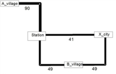
Image 160: Network volume for timetable-based assignment (parameter file timetab1.par)