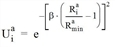
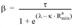
The model is described in Schnabel and Lohse (1997) and differs from the Lohse model in that the distribution parameter β is determined depending on the value of the minimum impedance Rmina. The calculation can be calibrated in more detail when using three additional parameters τ, λ and κ.
The following approach applies:
The following therefore applies:

β is calculated according to the following formula:
The impedance is additionally divided by a scaling divisor.
The variable distribution parameter β improves the modeling of the impedance sensitivity. Identical ratios of impedances are considered differently for short routes compared to long routes. In the case of two routes with impedances of 5 and 10 minutes or 50 and 100 minutes, the distribution is not the same.
The following example illustrates the effect of the distribution model Lohse with variable beta. In Image 94, different best paths (10 min, 50 min, 150 min, 300 min) are compared with "detour" alternatives. The distribution to the routes is done on the basis of the sumptuary ratio and the absolute value of the best path.
For shorter best paths and their alternatives lower detour sensitivity is assumed than for longer best paths.
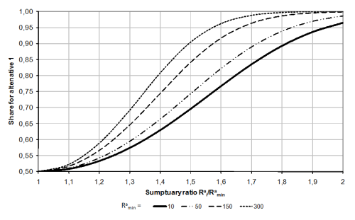
Image 94: Distribution with variable beta according to the modified Kirchhoff rule (see Schnabel / Lohse)
The parameters in Image 94 are described in Table 124.
|
τ |
λ |
κ |
Rmina |
β |
|
10 |
0.800 |
0.010 |
10 min |
3.32 |
|
10 |
0.800 |
0.010 |
50 min |
4.26 |
|
10 |
0.800 |
0.010 |
150 min |
6.68 |
|
10 |
0.800 |
0.010 |
300 min |
9.00 |
Image 95 shows the parameterization of the Lohse distribution model with variable beta on the interface.

Image 95: Parameterization of the Lohse distribution model with variable Beta
