This method computes an equilibrium assignment over a given assignment period, given both time-varying demand and time-varying supply.
Input – Supply
The available network is defined as usual by nodes, links, turns, zones, and connectors (optionally also main nodes and main turns). The attributes listed in Table 146 are relevant for DUE.
|
Network object |
Attribute |
Optionally time-varying |
Comment |
|
Link |
TSysSet |
No |
|
|
Length |
No |
|
|
|
v0 PrT |
Yes |
|
|
|
Capacity PrT |
Yes |
in [veh/h] |
|
|
Toll_PrTSys |
Yes |
|
|
|
DueVWave |
No |
See below for explanation of link impedance |
|
|
DueFunDiag |
No |
||
|
SpacePerPCU |
No |
||
|
LinkSpacePerPCU |
No |
||
|
Out capacity PrT |
Yes |
in [veh/h] |
|
|
Link type |
vMax_PrTSys |
No |
Maximum speed per transport system on any link of this type |
|
Turns |
TSysSet |
No |
|
|
t0 PrT |
No |
|
|
|
Capacity PrT |
Yes |
in [veh/h] |
|
|
Main turn |
TSysSet |
No |
|
|
t0 PrT |
No |
|
|
|
Capacity PrT |
No |
in [veh/h] |
|
|
Zones |
SharePrTOrig/Dest*) |
No |
Do connectors have shares{Yes/No} |
|
Connectors |
t0_TSys |
No |
|
|
Weight*) |
No |
Connector share if enabled for zone |
- *) with MPA only
Some of the attribute can be temporarily restricted. These attributes will then have a default value, but may assume a different value during a given interval within the assignment period.
The transport system set and the connector shares have the same meaning as in all other assignment methods.
Impedances are handled in a special way in DUE (Network performance model). In particular, link travel time is the sum of t0 with free flow and a wait time at the bottleneck which is assumed to be located at the end of the link. The free-running travel time t0 depends on a flow-density fundamental diagram. The fundamental diagram can have one of two different shapes which differ in the sub-critical branch, this means, where density is less than the critical density (at which maximum flow is reached). The shape is defined by the link attribute DueFunDiag.
In the case of urban links, a trapezium shaped fundamental diagram is recommended. In this type of diagram, the hypocritical branch is linear, which means that vehicles travel at free-flow speed v0 (on the free-running part) until capacity is reached. Image 134 illustrates how the shape of the diagram is determined by the link attributes.
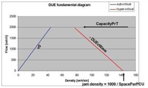
Image 134: Shape of the fundamental diagram based on link attributes
Notice that the jam density is the maximum number of vehicles per 1 km of link length. For a single-lane link a typical value for SpacePerPCU would be around 7 m, resulting in a jam density of ~140 vehicles / km.
In order for the fundamental diagram to be well-defined, the sub-critical and hyper-critical branches must not overlap. Therefore the link attributes must satisfy the condition:
Capacity PrT • (1 / v0 + 1 / DueVWave) ≤ 1 000 / LinkSpacePerPCU
For freeway links, the assumption of constant sub-critical speed is not always justified, and an approach similar to volume-delay functions appears more suitable.
In this type of diagram, the sub-critical branch is parabolic (Image 135), speed decreases from v0 at free flow to 0.5 • v0 at capacity, and the flow-density curve reaches capacity with zero derivative. The validity condition for the attributes then becomes
Capacity PrT • (2 / v0 + 1 / DueVWave) ≤ 1,000 / LinkSpacePerPCU.
All other properties are identical to the sub-critical linear case.

Image 135: Parabolic sub-critical branch in the fundamental diagram
The wait time at the end of the link is a function of the bottleneck capacity. This is defined for each turn by turn attribute Capacity PrT. To work correctly with DUE, turn capacities should be determined in the following way:
- First, determine the saturation capacity of each lane of the upstream arc, as the lane capacity multiplied by the green time fraction (g/c) corresponding to that lane in the case of a signalized intersection, or by some suitable multiplier in case of non-prioritized approach at a non-signalized intersection.
- Then, determine each turn capacity as the sum of the capacities of lanes allowed for the corresponding maneuver.
|
Note: In case of lanes allowed for more than one maneuver, the corresponding lane capacity is not to be split among the corresponding turns, but is to be entirely assigned to each turn corresponding to the allowed maneuvers. In this case in fact, DUE will, based on the turn flows resulting from WDDTA, internally identify the actual capacity to be assigned to each turn. |
Example
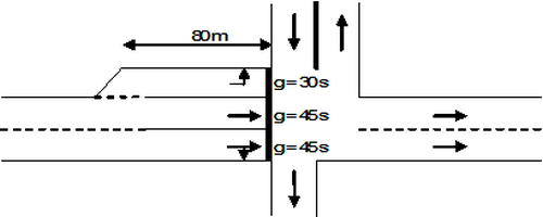
Image 136: Signalized intersection in reality
The signalized intersection in Image 136, with lane capacities = 1,800 veh/h, a signal cycle = 90 s, and green fractions, should be implemented in Visum as shown at the bottom of Image 137. The turns approaching from the West have the following capacities:
- turn 1 (1 lane allowed): Q1 = 1,800 • 30 / 90 = 600 veh/h
- turn 2 (2 lanes allowed): Q2 = 1,800 • 45 / 90 + 1,800 • 45 / 90 = 1 veh/h
- turn 3 (1 lane allowed): Q3 = 1,800 • 45 / 90 = 900 veh/h
Whereas the capacity of the right lane, which can be used to go either straight or right, is added both to the straight turn capacity and to the right turn capacity.
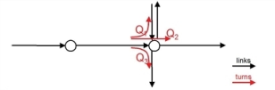
Image 137: Diagram of the signalized node in Visum
For the compensation of the turn capacity overestimation due to shared lanes the out capacity PrT of the incoming link from the West can be set, by adding up the saturation flow rate and the green ratio by lane for example:
S = 1,800 • 30/90 + 1,800 • 45/90 + 1,800 • 45/90 = 2,400
|
Note: For the PrT lane capacities and/or the link out capacity you can define time-varying values. In this way, you can model the effects of various green time splits depending on the time of day. |
Input – Demand
DUE accepts a description of time-varying demand. Like elsewhere in Visum, this description can take two possible forms:
- Total demand matrix with a demand time profile which assigns percentage shares of the total matrix to time intervals.
- A demand time profile in which each time interval refers to a different demand matrix.
If the assignment time period including the post-assignment period exceeds one day you need to use the calendar add-on.
DUE is a multi-class assignment method, this means, multiple demand segments, each with its own demand description, can be assigned in a single run.
An overview of all relevant input and output attributes for this procedure can be found under: ...\Program files\PTV Vision\PTV Visum 2022\Doc\Eng\AssignmentMethods.xls.
Output attributes of the Dynamic user equilibrium
The results of the operation are available through link, turn, main turn and connector attributes for volume and impedance. In particular, volumes are available as totals or by demand segment or transport system, and in vehicles, PCU, or persons. Both volumes and impedances are given by analysis time interval.
The definition of queue lengths as a measure of oversaturation is not easily defined, as in the DUE model queues may move and only gradually approach the situation where traffic is at a standstill at queue density. Because queues move (at a speed depending on the hyper-critical branch of the fundamental diagram), and separation between vehicles (density) is not constant, it would furthermore be misleading to speak of queue length in meters. Therefore we adopt a definition which is similar to “congestion hits” in more microscopic simulations. The value of the queue length (for a given link and time interval) is the number of vehicles experiencing hyper-critical delay, i.e. spend more time on the link than the free-running link travel time resulting from v0 plus the sub-critical wait time at the bottleneck (e.g. waiting for the next green time in the cycle).
