The Equilibrium_Lohse procedure is demonstrated below with a calculation example. Table 135 shows the parameter settings of Equilibrium_Lohse and the impedance for links and routes in the unloaded network. Table 136, Table 137, and Table 138 show three iterations of the calculation process.
|
LinkNo |
Type |
Length [m] |
v0 [km/h] |
Capacity [car units] |
R0* [min] |
|
1 |
20 |
5,000 |
100 |
1,200 |
03:00 |
|
2 |
20 |
5,000 |
100 |
1,200 |
03:00 |
|
3 |
20 |
5,000 |
100 |
1,200 |
03:00 |
|
5 |
20 |
5,000 |
100 |
1,200 |
03:00 |
|
6 |
20 |
5,000 |
100 |
1,200 |
03:00 |
|
7 |
20 |
5,000 |
100 |
1,200 |
03:00 |
|
8 |
30 |
16,000 |
80 |
800 |
12:00 |
|
9 |
30 |
5,000 |
80 |
800 |
03:45 |
|
10 |
40 |
10,000 |
60 |
500 |
10:00 |
|
11 |
40 |
5,000 |
60 |
500 |
05:00 |
Table 135: Impedance in unloaded network, input parameters of Equilibrium_Lohse procedure
|
Route |
Links |
Length [m] |
R0* [min] |
||
|
1 |
1+8+9 |
26,000 |
0:18:45 |
||
|
2 |
1+2+3+5+6+7 |
30,000 |
0:18:00 |
||
|
3 |
10+11+5+6+7 |
30,000 |
0:24:00 |
||
|
Input parameters:
|
|||||

|
LinkNo |
Volume 1 [car units] |
R1 [min] |
TT1 |
f(TT1) |
Delta ∆1 |
R1* [min] |
|
1 |
2,000 |
11:20 |
2.78 |
0.0452 |
0.4796 |
07:00 |
|
2 |
2,000 |
11:20 |
2.78 |
0.0452 |
0.4796 |
07:00 |
|
3 |
2,000 |
11:20 |
2.78 |
0.0452 |
0.4796 |
07:00 |
|
5 |
2,000 |
11:20 |
2.78 |
0.0452 |
0.4796 |
07:00 |
|
6 |
2,000 |
11:20 |
2.78 |
0.0452 |
0.4796 |
07:00 |
|
7 |
2,000 |
11:20 |
2.78 |
0.0452 |
0.4796 |
07:00 |
|
8 |
0 |
12:00 |
0.00 |
0.0450 |
0.5000 |
12:00 |
|
9 |
0 |
03:45 |
0.00 |
0.0450 |
0.5000 |
03:45 |
|
10 |
0 |
10:00 |
0.00 |
0.0450 |
0.5000 |
10:00 |
|
11 |
0 |
05:00 |
0.00 |
0.0450 |
0.5000 |
05:00 |
|
Route |
Volume 1 |
R1 |
R1* |
|||
|
1 |
0 |
0:27:05 |
0:22:45 |
|||
|
2 |
2,000 |
1:08:00 |
0:41:59 |
|||
|
3 |
0 |
0:49:00 |
0:35:59 |
|||
|
LinkNo |
Volume 2 [car units] |
R2 [min] |
TT2 |
f(TT2) |
Delta ∆2 |
R2* [min] |
|
1 |
2,000 |
11:20 |
0.62 |
0.0450 |
0.4925 |
09:08 |
|
2 |
1,000 |
05:05 |
0.27 |
0.0450 |
0.4962 |
06:03 |
|
3 |
1,000 |
05:05 |
0.27 |
0.0450 |
0.4962 |
06:03 |
|
5 |
1,000 |
05:05 |
0.27 |
0.0450 |
0.4962 |
06:03 |
|
6 |
1,000 |
05:05 |
0.27 |
0.0450 |
0.4962 |
06:03 |
|
7 |
1,000 |
05:05 |
0.27 |
0.0450 |
0.4962 |
06:03 |
|
8 |
1,000 |
30:45 |
1.56 |
0.0451 |
0.4855 |
21:06 |
|
9 |
1,000 |
09:37 |
1.56 |
0.0451 |
0.4855 |
06:36 |
|
10 |
0 |
10:00 |
0.00 |
0.0450 |
0.5000 |
10:00 |
|
11 |
0 |
05:00 |
0.00 |
0.0450 |
0.5000 |
05:00 |
|
Route |
Volume 2 |
R2 |
R2* |
|||
|
1 |
1,000 |
0:51:42 |
0:36:50 |
|||
|
2 |
1,000 |
0:36:45 |
0:39:22 |
|||
|
3 |
0 |
0:30:15 |
0:33:08 |
|||
|
LinkNo |
Volume 3 [car units] |
R3 [min] |
TT3 |
f(TT3) |
Delta ∆3 |
R3* [min] |
|
1 |
1,333 |
06:42 |
0.27 |
0.0450 |
0.4963 |
07:56 |
|
2 |
667 |
03:56 |
0.35 |
0.0450 |
0.4953 |
05:00 |
|
3 |
667 |
03:56 |
0.35 |
0.0450 |
0.4953 |
05:00 |
|
5 |
1,333 |
06:42 |
0.11 |
0.0450 |
0.4984 |
06:22 |
|
6 |
1,333 |
06:42 |
0.11 |
0.0450 |
0.4984 |
06:22 |
|
7 |
1,333 |
06:42 |
0.11 |
0.0450 |
0.4984 |
06:22 |
|
8 |
667 |
20:20 |
0.04 |
0.0450 |
0.4994 |
20:43 |
|
9 |
667 |
06:21 |
0.04 |
0.0450 |
0.4994 |
06:28 |
|
10 |
667 |
27:47 |
1.78 |
0.0451 |
0.4842 |
18:37 |
|
11 |
667 |
13:53 |
1.78 |
0.0451 |
0.4842 |
09:18 |
|
Route |
Volume 3 |
R3 |
R3* |
|||
|
1 |
667 |
0:33:23 |
0:35:07 |
|||
|
2 |
667 |
0:34:40 |
0:37:03 |
|||
|
3 |
667 |
1:01:47 |
0:47:02 |
|||
Table 135, Table 136, Table 137, and Table 138 illustrate the first three iteration steps of the Equilibrium_Lohse procedure for the example network.
Iteration step 1, n = 1
- Volume 1
The volume of the first iteration step results from an "all or nothing" assignment onto the lowest impedance route in the unloaded network. For impedance R0*, this is route 2 loaded with 2,000 car trips.
- Current impedance R1
The current impedance R1 of every link results from the BPR capacity function (a =1, b = 2, c= 1). For link 1, for example, the following can be calculated:
R1 (link 1) = 3 min x (1+(2 000/1 200)²) = 11 min 20s
- Estimated impedance R1*
The estimated impedance R1* of every link consists of the current impedance R1 and the estimated impedance R0* of the last iteration step. It results from the learning factor Δ. To determine R1* for link 1, the following calculations are necessary:
- R0* = 3 min = 180 s
- R1 = 11 min 20s = 680 s
- TT1 = |R1 - R0*| /R0* = |680 s - 180 s| / 180 s = 2.78
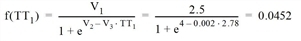
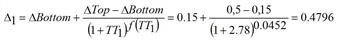
- R1* = R0* + Δ1 • (R1 - R0*) = 180 s + 0.4796 • (680 s - 180 s) = 420 s
Iteration step 2, n = 2
- Volume 2
The lowest impedance route for R1* is route 1. Now two routes exist, route 1 and 2. Each route is loaded with 1/n, i.e. ½ the demand, so that each route is used by 1,000 cars.
- Current impedance R2
The current impedance R2 of every link increases on newly loaded links 8 and 9, and it decreases on links 2, 3, 5, 6 and 7.
- Estimated impedance R2*
The estimated impedance R2* of every link consists of the current impedance R2 and the estimated impedance R1* of the last iteration step.
Iteration step 3, n = 3
- Volume 3
The lowest impedance route for R2* is route 3. 2,000 car trips are now equally distributed across routes 1, 2 and 3.
- Current impedance R3
The current impedance R3 again results from the current volume 3 via the VD function.
- Estimated impedance R3*
The estimated impedance R3* of every link consists of the current impedance R3 and the estimated impedance R2* of the last iteration step.
Iteration step 4, n = 4
The concluding route search based on R3* determines route 1 as the shortest route. Thus, the following route volumes result:
- Volume route 1 = 2/4 • 2,000 = 1,000 trips
- Volume route 2 = 1/4 • 2,000 = 500 trips
- Volume route 3 = 1/4 • 2,000 = 500 trips
