Table 141 shows the key input data used in the example network. If the following parameters are chosen for the search, then in a single external iteration, all 3 conceivable routes will be found:
- Number of search iterations = 5
- σ= 8 • R0.5
- Compared to the "objective" impedances (resulting from impedance definitions and VDFs), the impedances of the network objects are changed for alternative shortest path searches. They are drawn randomly from a normal distribution which has the objective impedance R as mean value and whose standard deviation σ is given as a function of R.
|
LinkNo |
Type |
v0 [km/h] |
Length [m] |
Capacity [car units] |
R0* [min] |
R0* [s] |
|
1 |
20 |
100 |
5000 |
1200 |
3:00 AM |
180 |
|
2 |
20 |
100 |
5000 |
1200 |
3:00 AM |
180 |
|
3 |
20 |
100 |
5000 |
1200 |
3:00 AM |
180 |
|
5 |
20 |
100 |
5000 |
1200 |
3:00 AM |
180 |
|
6 |
20 |
100 |
5000 |
1200 |
3:00 AM |
180 |
|
7 |
20 |
100 |
5000 |
1200 |
3:00 AM |
180 |
|
8 |
30 |
80 |
16000 |
800 |
12:00 PM |
720 |
|
9 |
30 |
80 |
5000 |
800 |
3:45 AM |
225 |
|
10 |
40 |
60 |
10000 |
500 |
10:00 AM |
600 |
|
11 |
40 |
60 |
5000 |
500 |
5:00 AM |
300 |
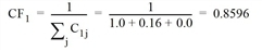
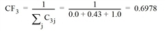
After completing the search, the correction factor for the independence of each route is determined according to Cascetta. It is based on the similarity of the individual route pairs with reference to time t0 or to the length. Table 142 shows the commonality factors C. These are used to calculate the correction factor CFr of route r.
- Route 1
- Route 2

- Route 3
The share by route is calculated from the correction factor according to Cascetta and from the impedance Rmin0 in the unloaded network.
For Route 1, the portion is calculated using the Logit model as follows:

In the same way, the shares for routes 2 and 3 shown in Table 143 are calculated. The product of share P and demand F is the volume of each route qr1 in the first iteration step. For Route 1, the calculation is as follows: 0.425 • 2000 = 849.4 PCU. Based on the route volumes, the link volumes and thus the network impedances can be calculated (Image 110). This results in the impedances R1 of the routes. These interim results can be reproduced in Visum if the maximum number of internal iterations are set to M = 1 in the assignment parameters.

Image 110: Volumes and link run times after the first internal iteration step m=1
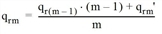
For the route choice in the second iteration step, an estimated impedance Rmin1 is calculated. Since Δ = 0.5, this impedance results from the formation of the mean value of Rmin0 and R1. On the basis of Rmin1, as in the first iteration step, the assignment is then made for the 3 routes. For each route, the interim result is qr2’. To smooth the volumes between two iteration steps, the MSA method (Method of Successive Averages) is used.
For m = 2, this results in the following for the volume of Route 1:
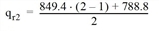
This route volume then leads to the link volumes and impedances of the second iteration step (Table 144). The iterations are repeated until the termination criteria are met.
