Since the eighties, primarily in English-speaking countries, so-called matrix correction (or matrix estimation) techniques have been used to produce a current demand matrix from an earlier travel demand matrix (base matrix) using current traffic count values. Based on research by Van Zuylen/Willumsen (1980), Bosserhoff (1985) and Rosinowski (1994) which focuses on matrices for private transport, PTV has extended the application of these techniques to public transport.
The starting point for the classic procedure is the travel demand for the individual OD pairs fij. Travel demand is usually described as a matrix, but for our purposes a vector representation containing all OD trips with non-zero demand is more suitable.
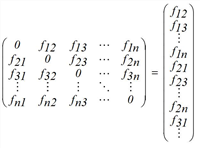
While it is usually assumed, that a matrix based on an earlier time is known, only partial information is provided for the current state. Important is the situation where there are no data based on relations (from an origin destination survey) available, but only count values at individual positions in the network. These can e.g. be origin / destination traffic or link volumes. We note the count values as another vector.
cr = (c1 c 2 c3 ... cm)
The demand of any OD pair contributes to count data. In the case of origin/destination traffic, for example, the boundary totals of the matrix to be estimated are known. Link volumes correspond to the total of all OD pairs that run along the link. In general, the following linear equation shows the relationship between demand and count values:
A • f = c
whereby A is called flow matrix. An element ask of A corresponds to the proportion of trips of OD pair k, which traverses the count object (e.g. the distance) s. For origin / destination traffic count values, A is especially constant, as specified with example n = 3, m = 6.
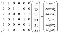
In this case, in particular, the proportional matrix A does not depend on the assignment. For link volumes, on the other hand, supply-dependent path selection is included in A. The flow matrix is obtained through the assignment of an existing matrix (for example, the old demand matrix) to the supply at the time of the count. Both types of count values can be also be used next to each other without a problem.
The problem with matrix correction is that the number of count objects is usually significantly smaller than the number of OD pairs m << n2, and thus the new matrix is under-determined by the count values. Out of the countless matrices which match the count values "match", only the best is selected according to a evaluation function q, thus solves the optimization problem:
max q(f), so that A • f = c
A combination of entropy and weighting with the proportions of the old matrix often serves as an evaluation function. The evaluation function implemented in Visum is:

whereby the  represent the values of the old matrix. q is non-linear, so the problem must be solved iteratively.
Image 62 shows for an example how the entropy changes depending on the estimated matrix value ƒij.
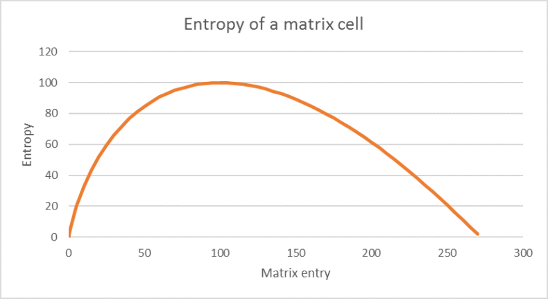
Image 62: The entropy of a matrix entry whose original value is 100. The maximum entropy is reached if the matrix entry is identical to the original value.
In this wording of the matrix correction problem there is, however, another weakness of the classic approach: vector c of the count values is assumed as a known parameter, free of every uncertainty. A q maximum is only selected from the matrices which fulfill the exact secondary conditions. The count values thus receive an inadequate weight, because each survey provides a snap shot, which is afflicted with a statistical uncertainty. Conventional procedures (for example from Willumsen) do not allow such a state, because the count values are perceived as "strict" secondary conditions.
PTV has therefore taken on the approach by Rosinowski (1994), who modeled the count values as fuzzy measured data similarly to the Fuzzy Sets Theory. If it is known that in a zone, the origin traffic fluctuates up to 10 % from day to day, in other zones however about 25 %, this is illustrated with the respective tolerances t. In the secondary conditions of the matrix estimation problem, thus fuzzy conditions with different tolerances replace strict values.
This is achieved by introducing non-negative slip variables r and s which replace the original secondary with:


In this case, the vectors  and
and  Are defined by
  and
and  , t is the tolerance vector.
If one left it at that, all results between  and
and  all results would be allowed and evaluated equally, irrespectively of whether they are in the middle or at the edge of they are in the middle or at the edge of an interval. In reality, however, one favors a result in the middle of the permitted interval, because then the count value would be hit exactly. This ideal case occurs when r = s = t.
Thus for the slip variables r and s corresponding entropy terms are added to the weighting function, whereby the tolerances t serve as weighting variables:

By illustrating the entropy of the slip variables in an example, you can see its similarity to fuzzy sets.
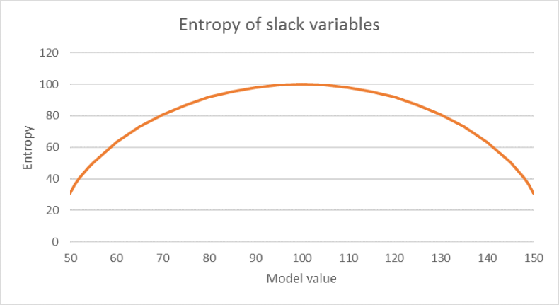
Image 63: For example, imagine a count value of 100 with a tolerance of 50. The model value is a value of the vector A•ƒ.
The entropy of the slip variable becomes maximum if the count value is exactly hit, otherwise it decreases towards the edges. This corresponds to a fuzzy set with the interval [50, 150] as the carrier set and the above-mentioned membership function.
An illustration using fuzzy conditions in contrast to strict limits thus makes it possible to express the preference for central values within the carrier set. This means that values close to the mean value of the count values are generally preferred, but values at the edge are also accepted if this results in a significantly smaller deviation from the count values.
The range of solutions of the estimate problem expands due to the Fuzzy-similar formulation, and with the degree of freedom for entropy maximization increases, so that generally higher target function values can be achieved. To make it clearer, the "most likely" demand matrix is thus estimated, which represents the count values within the ranges of fluctuation.
