Image 53 depicts the calculations for the absolute and incremental form.
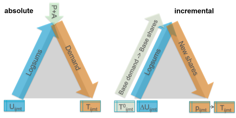
Image 53: Calculation for the absolute and incremental form
The triangles shown against a gray background represent model structures without specifically naming the choice on the levels. The calculation is generally performed as depicted by the colored arrows:
- In both cases – absolute and incremental – the logsums are calculated in hierarchical order (starting at the bottom) and then passed on to the next level until the top is reached. With the absolute form, you need to enter utilities for the lowest leaf node of the model structure. With the incremental form, you require the utilities of the base case as well as of a scenario in order to determine utility changes for the calculation of logsums. Please note: The values of the utilities must be smaller than or equal to zero if you use the Nested demand gap calculation procedure.
- To recalculate the demand (absolute form) with destination choice, you need productions and attractions (P+A), which are entries on the level of destination choice. By default, these values are expected in the zone attributes productions (<DStrCode>) and attractions (<DStrCode>). Only with coupling across demand strata, i.e. when multiple demand strata use the same destination potential, do you have to save the values to a user-defined zone attribute.
- To recalculate the demand (absolute form) without destination choice within the Nested demand procedure, e.g. during a solely nested mode choice, you must specify input matrices, i.e. it is assumed that a destination choice has already been computed.
- With incremental calculation, demand shares of the base demand are calculated in hierarchical order, starting at the bottom of the leaf nodes, and are then aggregated accordingly to the top level. Matrices are always required as base demand at the leaf nodes.
Calculation for the absolute model form
In the following, we will take a look at the model structure in the form of a decision tree with nodes. Each node has one or multiple child nodes that represent the alternatives. The calculation is carried out individually for each origin zone.
Let node N be a node with a number of child nodes N1,…,NJ. At node N there are a scaling factor λN and an alternative-specific constant ASCN The ultility of the child nodes Nj shall be  .
.
If a mode or time of day choice takes place at node N (i.e. the child nodes N1,…,NJ are either mode nodes, nest mode nodes or time of day nodes), then the utility of node N is determined by:

If the choice type at node N is destination choice (i.e. the alternatives at the child nodes N1,…,NJ are the destination zones), then the utility of node N is given by:

Aj is the destination potential of zone j.
When calculating demand, a distinction is also made according to the type of choice. Let TN be the demand at node N. If the choice type at node N is mode choice or time-of-day choice, then the demand  at child node Nj is given by:

If the choice type at node N is destination choice, then the demand at child node Nj is given by:
 .
.
Calculation for the incremental model form
At the lowest level of the leaf nodes, instead of the the utility U(Scenario), incremental calculation uses the the utility difference ∆U = U(Scenario) - U(Base) between the scenario and base case. In the first step, the utility differences are calculated upwards from the lowest level. The utility difference of the child nodes Nj is  .
.
The demand at the child nodes Nj in the base case is  . The demand at node N in the base case is
  and the share of demand in the base case shall be
  . Then the utility difference of node N is given by:
 .
.
In the second step, the demand is calculated from top to bottom in the tree. Suppose there is a demand of TN at node N. This results in a demand  at child node Nj given by:
