Choice models for boarding decisions
In the headway-based assignment it is usually assumed that passengers know line headways and times.
Which additional information they have, is decisive for their choice behavior when boarding or transferring. Visum offers four different models:
- No information and exponentially distributed headways
- No information and constant headways
- Information on the elapsed wait time
- Information on the next departure times of the lines from the stop
The latter applies for example, when dynamic passenger information systems have been installed at stops. The passengers can then see which of the departing lines in the current situation offer the least remaining travel time to their destination. As a result, they will for example not board a line if the information system gives them the information, that shortly after this line there will be another much faster line.
Notation
L = {1, ..., n} describes the set of available PuT lines. Each line i ∈ L has a certain remaining journey time si ≥ 0 and a headway hi > 0. The frequency  of the line is derived from the latter. The term "remaining" should make it clear that we are talking about the remaining journey time from the currently considered stop to the destination zone. Only for the choice situation at the origin zone we are talking about the journey time of the entire path.
For the purpose of a more simple modeling we assume additionally that the lines are sorted in ascending order according to their remaining journey time. Thus the following applies s1 ≤ s2 ≤ ... ≤ sn. The set of the first i lines is coded as follows: Li = {1, ..., i}.
Note, that the remaining journey time si in fact stands for the generalized costs of line i, which contain transfer penalties and further impedance components. For a better understanding we will still be talking about "Times".
On the basis of the available information the different choice models calculate the optimal set L* ⊆L and for each line i ∈ L* a demand share πi ≥ 0.
It is clear that a line i must be part of L* if another line j is contained in L* and if si < sj applies for the remaining journey times. From sorting the times it can be deducted that i* exists, as a consequence L* = Li*.
The wait time which applies when choosing any set L‘ before boarding, is designated as WL‘. The respective remaining costs are given as follows.
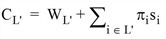
The parameters are random variables because they depend on the random arrival of lines at the stop.
For the optimal set L* the following also applies: E(CL*) ≤ E(CL‘) for any L‘ ⊆L.
