This model is based on the assumption that a passenger does not only know the times and headways of all lines, but can (at least at the stop) also get information on precise departure times. The optimal strategy can thus be formulated as follows.
A passenger boards the line that offers the least remaining costs given the actual departure times.
Unlike in previous cases, the passenger does not simply board the first arriving line of a certain (possibly time dependent) set. Because all wait times wi are known, the passenger's decision is not subject to stochastic influences. He or she rather selects exactly that line whose remaining costs si + wi are at a minimum.
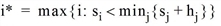
The optimal line set thus consists of all lines, which have the least costs in some timetable positions.
 and
and 
The optimal set of lines are those, which are optimal in border cases, since they arrive without a wait time, whereas all other lines have to be waited for by a complete headway.
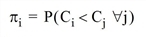
The calculation of shares is as follows.
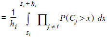 [60.4]
Explanation of the derivation
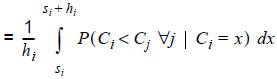
In row [60.1], the entire passenger information is used. Line i is selected if its remaining costs Ci are lower than those of the other lines. Row [60.2] reformulates the expression, by using the density function of the random variable Ci. Due to constant headways Ci is equally distributed in [si,si + hi). (If the wait time is weighted with a factor, this should be put in front of hi, the calculation otherwise does not change.)
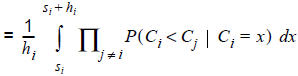
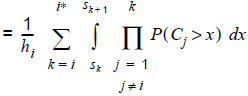
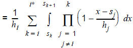
In row [60.3] we take advantage that the departures of the lines are independent of each other. In all choice models this is a basic assumption of the headway-based assignment. To avoid case differences, the integration range in [60.5] is separated into sections, in which the inner product is extended over a constant set of lines. It has to be noted that for j > k and x ∈ [sk,sk+1) the following must apply: P(Cj > x) = 1. This is due to the sorting of the lines at the beginning, because the costs of line j > k sum up to at least sk+1. In the last step [60.6] we then apply the distribution function of Cj which again is an equal distribution. At the end of the invoice, the result is a sum of polynomials with a maximum degree of i*.
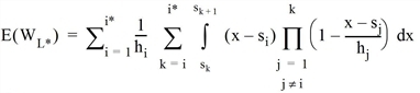
The expected wait time is achieved analogously.
To assume passenger information is no extremely strict requirement. Many places already have information systems which display the next departure times on the basis of real-time operating data. Alternatively, timetables could be hung up at stops. There are also no limits regarding other technical resources.
