Headway calculation
For the PuT supply displayed in Image 157 the headway-based procedure determines the headways for the analyzed time interval from 05:30 a.m. to 07:30 a.m. (120 minutes) illustrated in Table 178 – if these are calculated according to the method from mean headway (Headway calculation).
|
Line |
Mean follow-up time |
Headway |
|
Bus 1 |
120 / 3 * = 40 min |
40 min |
|
Train |
120 / 2 ** = 60 min |
60 min |
|
* 3 departures in analyzed interval (6:10, 6:55, 7:25) from A-Village ** 2 departures in analyzed interval (6:25, 7:05) from Station |
||
Route search
The case is, that passenger information on departure times exists and is also available on board of the bus line. The procedure will then determine two routes when searching for a route from A-Village to X-City if both alternatives are better than the respective other with positive probability.
- Route 1 (bus 1, no transfer) and
- Route 2 (bus 1 and train, 1 transfer)
Probability becomes involved in that the wait time for the train in the case of a transfer is within a range of between 0 and 60 minutes and no fixed transfer time has been assumed in advance.
If no extremely high transfer time penalty is used, some of the passengers will certainly use the transfer option. This is because the train will leave (with a certain level of probability) only shortly after the bus arrives and the passengers will thus arrive at their destination more quickly.
Because the probability of obtaining an unfavorable connection in this case is significantly higher, however, the majority of the passengers will continue their journey by bus.
The decisive factor is thus not only the mean wait time for the train – in the example given, this is 30 minutes – but the complete range of possible wait times. Due to the existing passenger information, each of the two routes thus receives precisely that portion of the demand that corresponds to the chance of being the better of the two options.
Route choice
In order to determine a distribution in the example given, specific impedance parameters have to be used. These are set as follows.
- Imp = PJT • 1.0 + number fare points • 0.0
- Perceived journey time PJT = in-vehicle time • 1.0
+ Access and egress time • 1.0
+ Walk time • 1.0
+ Origin wait time • 1.0
+ Transfer wait time • 1.0
+ Number of transfers • 2 min
In this way, the impedances listed in Table 179 are calculated for a passenger arriving at the railway station on Bus 1 for the remaining route legs.
From the impedances Imp1 and Imp2, the following percentages P1 and P2 of the OD demand (in this case: 90 trips) result and thus the absolute number of trips on both routes (M1 or M2). This occurs as follows.
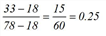
The decision as to which of the routes is more attractive depends on whether the random variable Imp2 is greater or smaller than the constant variable Imp1. Because Imp2 is uniformly distributed in the interval [18, 78[ and Imp1 is equal to 33, the probability for choosing Route 2 is thus 0.25 according to the formula below.
This means that 90 • 0.25 = 22.5 passengers decide to travel by train and 90 • 0.75 = 67.5 passengers to continue their journey by bus.
This results in the volumes shown in Image 157.
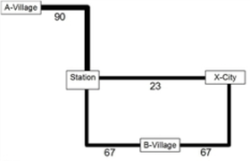
Image 157: Volume for headway-based assignment, transfer penalty 2 min
With any variation in the transfer penalty, this portion changes as shown in Table 180. For other impedance parameters, the same applies.
The skim values for the relation from A-Village to X-City are shown in Table 181. These values are the mean skim data of both routes which – weighted with the number of passengers – are summarized for the impedance parameters used here.
Please pay particular attention to the transfer wait time of 7.5 minutes for Route 2. In this case, the figure is not 60 / 2 = 30 minutes even though the train's headway is 60 minutes. This is due to the fact that passengers will only take the train if the transfer wait time is short enough – to be precise, when this time (as seen above) is within a range of zero and 15 minutes. In all other cases, there is no benefit in transferring. The 7.5 minutes transfer wait time in the choice of Route 2 therefore represents a conditional expectancy value – it is the mean wait time for those passengers for whom Route 2 is in fact the best alternative.
