Basics of assignment with toll consideration
The decisive feature of an assignment procedure is the impedance definition for route evaluation and route choice. In all toll-regarding assignment procedures, the impedance Rr of a route r consists of travel time tr and monetary costs cr:

Here, VT is the value of time in [€/h], for example. Though this equation applies to all toll-regarding assignment procedures, the TRIBUT procedure differs from other procedures in two properties:
- Monetary route costs can be calculated in different ways.
- The value of time VT is no constant value per demand segment, but VT is modeled as stochastic parameter that varies according to a particular probability distribution.
|
Note: In the context of TRIBUT procedures, it does not make sense to include the toll in the definition of impedance because TRIBUT takes the amount into account via the time value settings in the assignment parameters. |
Link toll
In the simplest case, the route's monetary costs result from summing up the toll amounts by link along the route.
The following applies:
|
tL = t(VolL) |
Travel time on a link L as a function of the volume |
|
VolL |
Volume of link L |
|
CL |
Toll value for using link L |
|
VT |
Value of time in [€/h], for example |
The German HGV toll, for example, is a link toll. For trucks, a toll is charged on part of the network (highways and federal roads) that is exactly proportional to the distance traveled. Thus to each link of the highway and federal road link types the product from the link length x constant km cost multiplication can be allocated as toll amount. For any other link and for any other transport system, the toll amount = 0. The total of these amounts summed up along a route represents the cost resulting from the distance traveled on highway and federal road links for the transport system HGV.
For link toll, no toll system has to be defined. It is not necessary either to include the link attribute Toll-PrTSys in the impedance definition, since TRIBUT regards this amount automatically.
|
Note: The TRIBUT-Equilibrium assignment always regards the link-specific toll values. The TRIBUT-Equilibrium_Lohse procedure only regards the link-specific toll values of links which do not belong to any toll system. |
Area toll
Especially toll systems for inner city areas often use a different type. For the area toll, a geographically coherent section of the network is stated as toll area. A fixed amount, independent of the distance, is charged if a route leg runs through the toll zone:
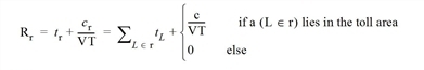
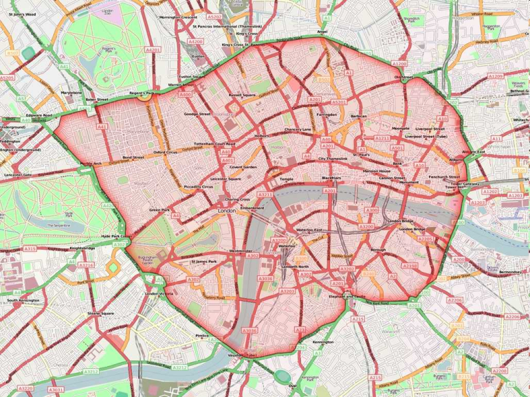
Image 107: Example for area toll: The London Congestion Charging Zone
At first view, the monetary costs of a route do not depend on the individual links being traversed, but on the route course as a whole in this case. Basically this is right, however, TRIBUT - like any other assignment procedure - is based on shortest path searches via links and requires the impedances by link therefore. That is why TRIBUT puts the area toll down to the link toll case. For that, define the toll area first by creating a network object 'toll system' of the area toll type and then allocating the toll area's number to all links which are located in the area as value for the attribute Toll system number. The toll system additionally stores the fixed toll amount for each transport system. For the clear definition of the figure described below, all connector nodes of a zone need to be located either within the toll area or outside of it.
On this basis, TRIBUT defines the toll amounts for links, turns, and connectors as follows:
cL = 0 for all links L
cC = 0 for all connectors C
 for all turns T, with δT = 1 if turn T leads from a link inside the toll area to a link outside or vice versa, i.e. if the toll area border is crossed. Otherwise, δT = 0.
 for all transitions X from connectors to links, where δX = 1 if the transition X leads to a link in the toll area or originates from there. Otherwise, δX = 0.
Image 108 illustrates the principle:
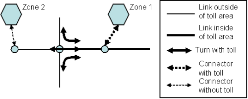
Image 108: Reducing area toll to link toll (for reasons of clarity, turns without toll are not displayed)
Summing up the toll amounts along a route results in an amount null for routes that do not touch the toll area at all. Any other route (origin traffic, destination traffic, through traffic, internal traffic of the toll area) is charged with the toll amount of c since they traverse exactly two network objects with toll amount = c/2 each.
In a Visum model, you can define multiple toll systems of the area toll type. Then, the definitions for turn and connector cost are applied to each toll system with the associated fixed toll amount. For turns between two toll areas, the two toll amounts are charged.
Please note the two characteristics. For routes, that cross the border of the toll area multiple times the toll amount is charged multiple times. This might not correspond to reality, however, it cannot be avoided for the required reduction to additive toll amounts per network object. Furthermore, the internal traffic within the toll area can be excluded from toll calculations in reality. For the TRIBUT route choice it is no problem that these flows are nevertheless charged with toll amounts, since the toll comparably refers to all route alternatives and thus this additive constant value does not modify the equilibrium solution. But when calculating a skim matrix of the impedance for future use in a demand model for example, you need to perform an additional matrix operation after skim matrix calculation to subtract the toll amount from the internal traffic OD pairs data.
|
Note: Only the TRIBUT-Equilibrium_Lohse procedure takes the area toll into consideration. For links that belong to a toll system the link attribute Toll-PrTSys is not regarded. |
Matrix toll
Another type of toll models is often applied to arterial highways. A subset of links is designated as a toll zone with a small number of connections (entries and exits) to the rest of the network (Image 109).
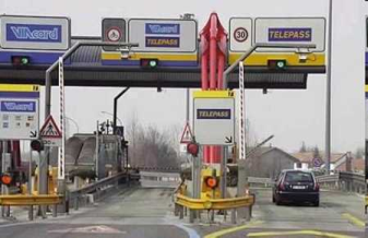
Image 109: Toll station at highway exit
Toll amounts are not defined as the sum of toll amounts by link, but arbitrarily as fee by pair (entry, exit). Using such a fee matrix, the operator has more flexibility since the toll amounts for longer routes can be defined irrespectively of the toll amounts for shorter sections of a longer route. Usually, those tariffs are on a diminishing scale, thus the rate per kilometer declines with increasing total distance.
As a matter of principle, such a matrix toll (which is named according to the fare matrix) cannot be reduced to summing up the toll amounts by link. Let's have a look at the example in Image 110:
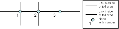
Image 110: Example of a matrix toll
The links 1-2 and 2-3 form a highway corridor with matrix toll. For that, define the toll area first by creating a network object 'toll system' of the matrix toll type and then allocating the toll area's number to all links which are located in the area as value for the attribute Toll system number. The toll system additionally contains a matrix of toll amounts per transport system for the roads between all border nodes of the toll area. In our example, these are the nodes 1, 2, 3. The toll amounts are listed in Table 143.
|
from / to node |
1 |
2 |
3 |
|
1 |
0 |
2 |
3 |
|
2 |
2 |
0 |
2 |
|
3 |
3 |
2 |
0 |
Please note, that the toll amount for the overall link is less compared to the two individual links.
For each pair (entry, exit) in the toll area, TRIBUT generates a virtual link with the toll amount from the matrix in the network and uses these virtual links for the shortest path search. In contrast, the original links in the toll area are not regarded for the shortest path search. For travel time computation, the volumes by virtual link are transferred back to the original links. This allocation is always based on the route with the minimum time (regarding t0) required between 'from node' and 'to node' of the virtual link. Image 111 shows the graph that is generated for the shortest path search in the example.
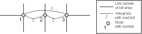
Image 111: Shortest path search graph with matrix toll
This modeling approach assumes a degressive toll matrix, i.e. if there are three nodes A, B, and C, always cA-C ≤ cA-B + cB-C. Furthermore, the number of virtual links that are added to the search graph exhibits quadratic growth proportionally to the toll area's number of border nodes. Thus you should use a toll matrix only in those cases where the toll area is connected to the surrounding network by a manageable number of nodes.
In a Visum model, you can define several toll systems of the matrix toll type. Nevertheless, each link may belong to just one toll system.
|
Notes: Only the TRIBUT-Equilibrium_Lohse takes the matrix toll into consideration. For links that belong to a toll system the link attribute Toll-PrTSys is not regarded. |
The Value of Time as stochastic parameter
Additionally, the TRIBUT procedure features the definition of the value of time (VT) and the impact of this definition (Table 144). This description is reduced to the link toll case, since the basic principle does not differ by toll type.
The complexity of a bicriterial route choice procedure is illustrated in a time-cost diagram:
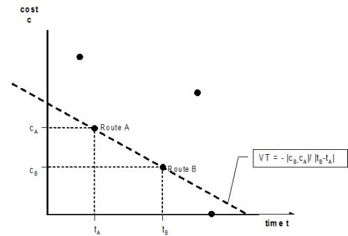
- Each point on the diagram, for example A = (tA,cA), corresponds with a route of the same origin destination relation.
- A certain time value VT corresponds with a family of parallel straight lines with a negative slope.
- If two routes lie on one VT straight, they are ”equally good” (for a user with the same VT). This VT is also characterized as a critical VT for two routes.
