Introductory example of equilibrium assignment

The effectiveness of the equilibrium assignment is described in the example in Table 129 and Image 92. The example analyzes the relation between traffic zone "village A" and traffic zone "city X".

The total impedance of a route, for the sake of simplicity, results from the sum of link impedances of the route (Impact models). Impedances for connectors and turns are not considered in the route search. In detail, the following assumptions apply:

• The impedance of the links is determined from the current travel time tCur. The current travel time tCur is in turn calculated using the capacity restraint function BPR with a=1, b=2 and c=1.
• The access and egress times for the connectors are not considered, that is, they are set to 0 minutes.
• Turn penalties are not considered.

With regard to the traffic demand the following applies.

• The traffic demand between A-Village and X-City is 2,000 car trips during peak hour.
• Capacity and demand refer to one hour.

The example network contains three routes which connect village A and city X.

• Route 1 via nodes 10 – 11 – 41 – 40
• Route 2 via nodes 10 – 11 – 20 – 21 – 30 – 31 – 40
• Route 3 via nodes 10 – 12 – 21 – 30 – 31 – 40

Route 1 mainly uses country roads and is 26 km long. It is the shortest route. Route 2 is 30 km long. It is the fastest route because the federal road can be traversed at a speed of 100 km/h if there is free traffic flow.

Route 3 which is also 30 km long is an alternative route which only makes sense if the federal road is congested.

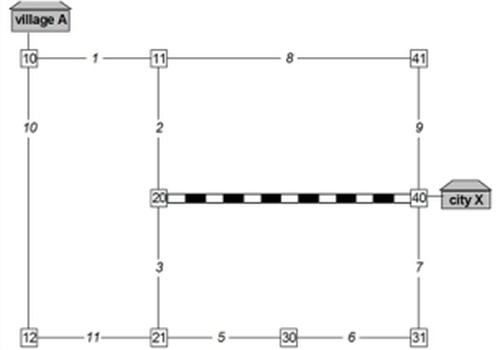
Image 92: Example network for equilibrium assignment

Table 129: Example network for equilibrium assignment

LinkNo	From Node	To Node	Type	Length [m]	Capacity [car units/h]	v0-PrT [km/h]
1	10	11	20 Federal road	5000	1200	100
2	11	20	20 Federal road	5000	1200	100
3	20	21	20 Federal road	5000	1200	100
4	20	40	90 Rail track	10000	0	0
5	21	30	20 Federal road	5000	1200	100
6	30	31	20 Federal road	5000	1200	100
7	31	40	20 Federal road	5000	1200	100
8	11	41	30 Country road	16000	800	80
9	40	41	30 Country road	5000	800	80
10	10	12	40 Other roads	10000	500	60
11	12	21	40 Other roads	5000	500	60

As a result, the assignment provides values of Table 130 for the three routes (PrT paths).

Table 130: Assignment results for the three PrT paths

Route	tCur	Impedance	Volume (AP)
1	46min 39s	2798	1157.488
2	46min 34s	2794	618.079
3	46min 12s	2772	224.432

The most important assignment results for links are displayed in Table 131.

Table 131: Assignment result at the links

Link	tCur	Impedance	Volume (AP)	Saturation PrT (AP)	VehicleHr(tCur)	VehKmTravelled PrT
1	11min 40s	700	1908	170	370h 54min 19s	9537.839
2	5min 47s	347	1157	96	111h 43min 15s	5787.442
3	5min 47s	347	1157	96	111h 43min 15s	5787.442
5	7min 48s	468	1450	126	188h 29min 38s	7249.603
6	7min 48s	468	1450	126	188h 29min 38s	7249.603
7	7min 48s	468	1450	126	188h 29min 38s	7249.603
8	26min 35s	1595	750	110	332h 23min 38s	12001.270
9	8min 19s	499	750	110	103h 52min 23s	3750.397
10	15min 12s	912	292	72	74h 3min 56s	2924.321
11	7min 36s	456	292	72	37h 1min 58s	1462.161