HCM 2000 for Signalized Intersections
The signalized intersection methodology is documented in Chapter 16 of the HCM 2000.
The basic flow chart for performing capacity analyses for signalized intersections is displayed in Figure 59: Signalized intersection capacity analysis flowchart. You input the intersection geometry, volumes (counts or adjusted demand model volumes), and signal timing. The intersection geometry is deconstructed into lane (or signal) groups, which are the basic unit of analysis in the HCM method.
A lane (or signal) group is a group of one or more lanes on an intersection approach having the same green stage. For example, if an approach has just one pocketed exclusive left turn and one shared through and right turn, then there are usually two lane groups – the left and the shared through/right.
Figure 59: Signalized intersection capacity analysis flowchart
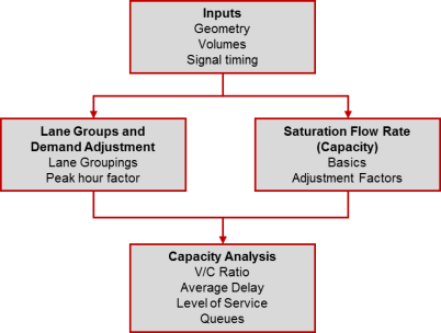
The volumes are then adjusted via peak hour factors, etc. For each lane group, the saturation flow rate (SFR), or capacity, is calculated based on the number of lanes and various adjustment factors such as lane widths, signal timing, and pedestrian volumes. Having calculated the demand and the capacity for each lane group, various performance measures can be calculated. These include, for example, the v/c ratio, the average amount of control delay by vehicle, the Level of Service, and the queues.
Step 1: Lane volume calculation from the movement volumes
This step distributes the movement volumes to lanes according to the user-defined geometry.
The basic distribution rule is to distribute the volumes uniformly to the lanes while taking the input movement volumes into account. You can overwrite a lane's utilization share within its lane group, if applicable.
Step 2: Volume adjustments by means of peak hour factors
The input lane volumes are adjusted to represent the peak hour volumes through the peak hour factor (PHF). The PHF is defined as:

Where
vh = hourly volume (veh)
v15 = peak 15-minute volume (veh)
Then,
vi = vg / PHF
where
vi = adjusted volume for lane group i
vg = unadjusted (input) volume for lane group g
PHF = peak hour factor (0 to 1.0)
Step 3: Calculation of de facto lane groups left/though/right
De facto lane groups are shared lanes with 100 m/h of their volume making one movement. For example, if a lane group is a shared left and through lane, and 100 % of the lane volume is making a left movement, then the lane group is converted to a de facto exclusive left lane group.
Step 4: Calculation of the types of left turns
The type of left turn needs to be determined in order to calculate the left turn adjustment factor.
The left turn type is set as follows:
1. Fully controlled if all turns of an approach are conflict free during their green times.
2. Fully secured if the left turns are conflict free during green time.
3. Fully secured + permitted if during green time left turns are first fully secured and then
permitted.
4. Permitted + fully secured if during green time left turns are first permitted and then fully
secured.
5. Without left turn stage, all other cases.
Step 5: Proportions of left turning and right turning vehicles by lane group
The proportion of right and left turn volume by lane group needs to be calculated.
PLT = vLT / vi
PRT = vRT / vi
where
PLT = proportion left turn volume by lane group
PRT = proportion right turn volume by lane group
vi = adjusted volume by lane group
vLT = volume of left turning vehicles by lane group
vRT = volume of right turning vehicles by lane group
Step 6: Saturation flow rate calculation by lane group
The saturation flow rate is the amount of traffic that can make the movement under the prevailing geometric and signal timing conditions. The saturation flow rate starts with an
ideal capacity, which usually is 1,900 vehicles per hour per lane (vphpl) for HCM 2000.
This number decreases due to various factors. The saturation flow rate is defined as:
si = (so)(N) • (fw)(fHV)(fg)(fp)(fa)(fbb)(fLu)(fRT)(fLT)(fLpb)(fRpb)
where
si = saturation flow rate of lane group i
so = ideal saturation flow rate per lane (usually 1,900 vphpl)
N = number of lanes in lane group
fw = factor for lane width adjustment
fHV = Heavy vehicle adjustment factor
fg = adjustment factor for approach grade
fp = adjustment factor for parking
fa = adjustment factor for the position of the link to city center (CBD true/false)
fbb = adjustment factor for bus stop blocking
fLu = adjustment factor for lane usage
fRT = adjustment factor for right turns
fLT = adjustment factor for left turns
fLpb = adjustment factor for pedestrians and bicyclists on left turns
fRpb = adjustment factor for pedestrians and bicyclists on right turns
First the description of the main calculation is described and then the various adjustment
factors are calculated.
Step 7: Calculation of actual green times
The effective green time (or actual green time for a lane group) needs to be calculated next.
The effective green time results as follows:
gi = Gi + li
gi = effective green time per lane group
Gi = green time per lane group
li = loss time adjustment per signal group
Step 8: Capacity calculation per lane group
Related to the saturation flow rate is the capacity. The saturation flow rate is the capacity if the movement has 100 % of the green time (this means, the signal is always green for the movement). The capacity, however, accounts for the fact that the movement must share the signal with the other movements at the intersection, and therefore scales the SFR by the percent of green time in the cycle. The capacity of a lane group is then defined as follows:
ci = si • (gi / C)
where
ci capacity i
si saturation flow rate i
C cycle time
gi / C green ratio i
Step 9: Calculation of the critical vol/cap ratio for the entire intersection
The critical v/c ratio of intersections is defined below. The HCM method is concerned with the critical lane group for each signal stage. The critical lane group is the lane group with the largest volume/capacity ratio unless there are overlapping stages. If there are overlapping stages, then the maximum of the different combinations of the stages is taken as the max. For the description of this method, please refer to HCM 2000, page 16-14, or HCM 2010, page 18-41.
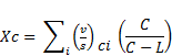
where
Xc = critical saturation (v/c ratio) per intersection
 = volume/capacity ratios for all critical lane groups
C = cycle time
L = loss time total of the signal groups of all critical lane groups
Step 10: Mean total delay per lane group
In addition to calculating the critical v/c per intersection, the mean delay per vehicle is calculated by the HCM method. The mean total delay is defined below.
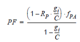
di = dUiPF + dIi + dRi
where
di mean delay per vehicle for lane group
dUi uniform delay
dIi incremental delay (stochastic)
dRi delay residual demand
PF permanent adjustment factor for coordination quality (see HCM 2000 "Signal coordination (Signal offset optimization)" on page 274)
where
dUi uniform delay for lane group i
gi effective (actual) green time
Xi = v/c volume/capacity ratio
Step 10b: Calculation of the incremental delay for each lane group
The incremental delay is the random delay that occurs since arrivals are not uniform and some cycles will overflow. It is calculated as follows:
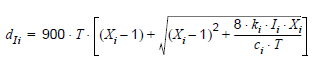
Where
dIi incremental (random) delay for lane group i
ci capacity for lane group i
Xi = v/c volume/capacity ratio
T duration of analysis period (hr) (default 0.25 for 15 min)
ki lookup value (HCM attachment 16 – 13) based on the controller type
Ii upstream filtering / metering adjustment factor (set to 1 for isolated intersection)
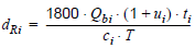
Step 10c: Delay calculation for the residual demand per lane group
The residual demand delay is the result of unmet demand at the start of the analysis period. It is only calculated if an initial unmet demand at the start of the analysis period is input (Q). It is set to 0 in the current implementation. It is calculated as follows:
where
dRi residual demand delay for lane group i
Qbi initial unmet demand at the start of period T in vehicles for lane group (default 0)
ci capacity
T duration of analysis period (hr) (default 0.25 for 15 min)
ui delay parameter for lane group (default 0)
ti duration of unmet demand in T for lane group (default 0)
Step 11: Delay calculation for the approach
The total delay per vehicle for each lane group can be aggregated to the approach and to the entire intersection with the following equations. The approach delay is calculated as the weighted delay for each lane group.
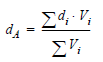
Where
dA mean delay per vehicle for approach A
di delay for lane group i
vi volume for lane group i
Step 12: Delay calculation for the intersection
The intersection delay is calculated as the weighted delay for each approach.
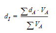
where
dI mean delay per vehicle for intersection I
dA delay for approach
VA volume for approach
Step 13: Level of Service calculation
The level of service is defined as a value which is based on the mean delay of the intersection (Table 24: Intersection Level of Service (LOS) for HCM 2000 Signalized Method).
Table 24: Intersection Level of Service (LOS) for HCM 2000 Signalized Method
|
Level of Service (LOS) |
Control Delay (s/veh) |
|
LOS A |
|
|
LOS B |
|
|
LOS C |
|
|
LOS D |
|
|
LOS E |
|
|
LOS F |
|


Step 14: Mean queue length calculation per lane group
Queue lengths are also calculated by the HCM 2000 method. The equation for the calculation of the mean queue length is as follows:
Q = Q1 + Q2
Where
Q = mean queue length: the maximum distance (measured in vehicles) that the queue extends on the average signal cycle
Q1 = mean queue length for uniform arrival with progression adjustment
Q2 = incremental term associated with random arrival and overflow to next cycle
Step 14a: Calculation of the number of residual vehicles after cycle 1
Q1 represents the number of vehicles that arrive during the red stages and during the green stages until the queue has dissipated.
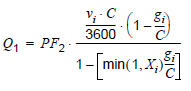
where
PF2 = progression factor 2
vi = volume of lane group i per lane
C = cycle time
gi = effective green time of lane group i
Xi = volume/capacity ratio of lane group i
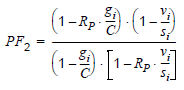
where
PF2 = progression factor 2
vi = volume per lane of lane group i
C = cycle time
gi = effective green time lane group i
si = saturation flow rate for lane group i
RP = platoon ratio: based on lookup table for arrival type
Step 14b: Calculate second-term of queued vehicles, estimate for mean overflow queue
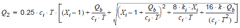
T = analysis period (usually 0.25 for 15 minutes)
k = adjustment factor for early arrival
Qb = initial queue at start of period (default 0)
ci = capacity for lane group i
k = 0.12 I • (sigi / 3600)0.7 for fixed time signal
k = 0.10 I • (sigi / 3600)0.6 for demand-actuated signal
I upstream filtering factor (set to 1 for isolated intersection)
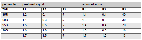
Step 15: Calculation of the queue length percentile
After calculating the mean back of queue, the percentile of the back of queue is calculated as follows:
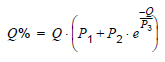
Where
Q average queue length
Saturation flow rate adjustment factors
We now return to the calculation of the saturation flow rate which involves several adjustment factors.
Step 6a: Calculate lane width adjustment factor
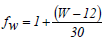
where
fw = lane width adjustment factor
W = mean lane width ( 8) (ft)
Step 6b: Calculate heavy goods vehicle factor
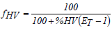
where
fHV = adjustment factor for heavy goods vehicles
%HV = percentage of heavy vehicles per lane group
EP = passenger car equivalent factor (2.0 / HV)
Step 6c: Calculate approach grade adjustment factor

where
fg = adjustment factor for approach grade
%G = approach grade as percentage (-6 % to +10 %)
Step 6d: Calculate parking adjustment factor
fP is calculated as follows:
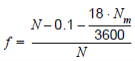
where
fp = parking adjustment factor (1.0 if no parking, else 0.050)
N = number of lanes in lane group
Nm = number of parking maneuvers per hour (only for right turn lane groups) (0 to 180)
Step 6e: Calculate adjustment factor for position to city center
fa = 0.9 if link is in the city center (CBD), otherwise 1.0
where
fa = adjustment factor for position
CBD indicates a central business district
Step 6f: Calculate bus stop blocking factor
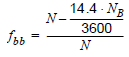
where
fbb bus stop blocking adjustment factor (0.05)
N number of lanes in lane group
NB number of bus stop events per hour (does not apply to left turn lane groups) (0 to 250)
Step 6g: Calculate lane utilization adjustment factor

where
fLu = adjustment factor lane utilization
vg = unadjusted (input) volume for lane group g
vgl = unadjusted (input) volume for lane with highest volume in lane group (veh per hour)
For this adjustment factor, an HCM lookup-table is regarded (HCM 2000: table 10-23 on page 10-26.
Step 6h: Calculate right turn adjustment factor
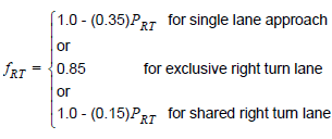
where
fRT right turn adjustment factor (0.05)
PRT proportion of right turn volume for lane group
Step 6i: Calculate left turn adjustment factor
The left turn adjustment factor is the most complex of the factors. The calculation is simple for protected left turns. However, if there is permitted phasing, then the equation is quite complex. It is as follows:
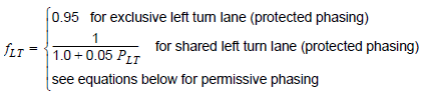
where
fLT = adjustment factor for left turns
PLT = proportion of left turn volume for lane group
For permitted staging, there are five cases. When there is protected-plus-permitted staging or permitted-plus-protected staging, the analysis is split into the protected portion and the permitted portion. The two are analyzed separately and then combined. Essentially this means treating them like separate lane groups. Refer to the HCM for how to split the effective green times among the protected and permitted portions.
1. Exclusive lane with permitted phasing: use the general equation below
2. Exclusive lane with protected-plus-permitted phasing: use 0.95 for the protected portion and the general equation below.
3. Shared lane with permitted phasing: use the general equation below
4. Shared lane with protected-plus-permitted phasing: use the equation above for protected phasing portion and the general equation below for the permitted portion
5. Single lane approach with permitted left turns: use the general equation below
The general equation for calculating fLT for permitted left turns is below. Note that this is not the exact HCM 2000 equation since there are a few different versions depending on the situation – shared/exclusive lane, multilane/single lane approach, etc. But the equation is similar regardless of the situation. This general equation is the equation for an exclusive left turn lane with permitted phasing on a multilane approach opposed by a multilane approach. The equation is basically the percentage of the time when lefts can make the turn times an adjustment factor. The adjustment factor is based on the portion of lefts in the lane group and an equivalent factor for gap acceptance time that is based on the opposing volume. The calculation of the percentage of the time when lefts can make the turn is a function of the opposing volume and their green time. The equation is as follows:
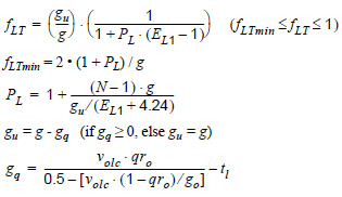
where
fLT = Global adjustment factor for left-turns
fLTmin = Minimum value for adjustment factor
g = Effective non-protected green time for left-turn lane group
gu = Effective non-protected green time for left-turns crossing a conflicting flow
PL = Share of left-turns using lane L
EL1 =Through equivalent for non-protected left-turns (veh/hr/lane) (look-up value depends on
conflict flow volume)
gq = Effective non-protected green time , while left-turns are blocked completely and the spill-back of the conflict flow is reduced
go = Effective green time for conflict flow
N = Number of lanes in lane group
Volc = Corrected conflict flow per lane per cycle = 
No = Number of lanes in the lane group of the conflict flow
vo = Corrected conflict flow
fLUo = Lane utilization factor for conflict flow
qro = Opposing queue ratio = max[1 - Rpo • (go / C), 0] (Rpo = look-up value depends on ArrivalType)
tl = Loss time for left-turn lane group
The opposing volume is calculated from the signal groups that show green while the subject lane group has green. To calculate the opposing volume for a subject lane group, the entire opposing volume is used even if there is an overlap.
The permitted left movement calculation does not need to be generalized to 4+ legs since only one opposing approach is allowed.
Step 6j: Calculate pedestrian adjustment factors for left and right turns
The computation of the factors for left-turning and right-turning pedestrians and bicyclists is a considerably complex operation. It is performed in four steps. For the computation, the bicycle volumes of the legs are regarded and the pedestrian volumes of the crosswalks. A traffic flow has potential conflicts with two crosswalks on the outbound leg. These two crosswalks head for the opposite directions.
NOTE: At a leg which is a channelized turn no conflicts occur between right turn movements and pedestrians.
Step 1: Determination of the pedestrian occupancy rate OCCpedg.
The pedestrian occupancy rate OCCpedg is derived from the volume. The following applies.
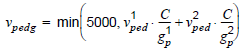
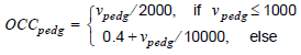
Here, vpedg is the pedestrian flow rate, v1pedg and v2pedg are the pedestrian volumes of the crosswalks, C is the cycle time of the signal control and g1p and g2p indicate the duration of the green for the pedestrians.
NOTE: In the HCM 2000 it is implicitly assumed, that the green for the left turn movements and the green for the pedestrians start at the same time. In Vistro, this is not the case, however. Thus, the following distinction of cases applies in Visum: If the pedestrian green time overlaps (or touches) the green or amber stage for vehicles, an existing conflict is assumed. In this case, the duration of the green of the pedestrian signal group is fully charged. Otherwise it is assumed, that there is no conflict. In this case, gp = 0 is assumed.
Step 2: Determination of the relevant occupancy rate of the conflict area OCCr
Here, three cases are distinguished:
- Case 1: Right turn movements without bicycle conflicts or left turn movements from one-way roads
In this case, the following applies:
OCCr = OCCpedg
Decisive for left turns from one-way roads is, that there is no opposite vehicle flow.
- Case 2: Right turn movements with bicycle conflicts
Here, straight turns of bicyclists are assumed.
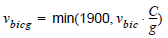
OCCbicg = 0.02 + vbicg / 2700
OCCr = OCCpedg + OCCbicg - (OCCpedg)•(OCCbicg)
Here, vbicg is the bicycle flow rate, vbic is the bicycle volume, C is the cycle time of the signal control, g is the effective green time of the lane group, and OCCbicg is the conflict area's occupancy rate caused by bicyclists.
- Case 3: Other left turn movements
These are left turn movements which do not originate from a one-way road. Here, a distinction of cases is made for the values gq and gp. gq is the clearing time of the vehicle flow on the opposite leg, and gp is the green time for the conflicting pedestrians. The following applies
gp = max(g1p, g2p)
- Case 3a: gq ≥ gp
In this case, the calculation is shortened, and the following applies
fLpb = 1.0
Pedestrians and bicyclists are irrelevant here, since the left turn movements have to wait until the vehicle flow on the opposite leg is cleared.
- Case 3b: gq < gp
The following applies
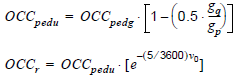
Here, OCCpedu is the occupancy rate of pedestrians after the clearance of the vehicle flow on the opposite leg, and OCCpedg is the pedestrian's occupancy rate.
Step 3: Determination of the adjustment factors for pedestrians and bicyclists on permitted turns ApbT
Here, two cases are distinguished with regard to the values Nturn – which is the number of lanes per turn – and Nrec, which is the number of lanes per destination leg.
- Case 1: Nrec = Nturn
Here applies ApbT = 1 - OCCr
- Case 2: Nrec > Nturn
Here, vehicles have the chance to give way to pedestrians and bicyclists. The following applies
ApbT = 1 - 0.6 • OCCr
Step 4: Determination of the adjustment factors for the saturation flow rates for pedestrians and bicyclists fLpb und fRpb.
fLpb is the adjustment factor for left turns, and fRpb is the adjustment factor for right turns. The following applies:
fRpb = 1 - PRT • (1 - ApbT) • (1 - PRTA)
fLpb = 1 - PLT • (1 - ApbT) • (1 - PLTA)
PRT and PLT represent the proportions of right turn and left turn movements in the lane group, and PRTA and PLTA code the permitted shares in the right and left turn movements (each referring to the total number of right turn and left turn movements of the lane group).