Defining links

Link attribute	Description	Values	Is native Visum attribute
No	ID of the link. Automatically set by Visum when a new link is added.	ID	YES
FromNodeNo	ID of the from node (node where the link starts). Automatically set by Visum when a new link is added.	Ref ID	YES
ToNodeNo	ID of the to node (node where the link ends). Automatically set by Visum when a new link is added.	Ref ID	YES
Name	Optional. Name of the link.	String	YES
Length	Length of the link.	[km]	YES
TsysSet	List of permitted transport systems on the link.	List	YES
NumLanes	Number of lanes on the link.	[n°]	YES
CapPrT	Maximum number of vehicles (PCU) that can enter the link in 1 hour. Important:  During the modeling activity, the CAPA value associated to a link cannot exceed the CapPrT value.	[PCU/h]	YES
V0PrT	Free flow speed on the link. Important:  This parameter is crucial in case Optima operates with real-time detected speed data. In this case, to ensure correct system behavior, perform a special calibration of the free flow speed parameter by analyzing a set of detected data.	[km/h]	YES
OutCapPrT	Optional. Maximum number of vehicles (PCU) that can exit the link in 1 hour.	[PCU/h]	YES
UseOutCapPrT	Define the link exit capacity. true: the link exit capacity is equal to OutCapPrT false: OutCapPrT is not relevant and the link exit capacity is determined as follows: In case of absence of head node geometry, it is equal to CapPrT In case of presence of head node geometry, see → Node model: detailed junction model	Boolean	YES
SpacePerPCU	Average space required by PCU per lane.	[m]	YES
DueVWave	Defines the slope for the hypercritical branch of the fundamental diagram.	[km/h]	YES
DueFunDiag	Defines whether the shape of the hypocritical part of the fundamental diagram is linear or parabolic.	[linear / parabolic]	YES
GREN	Optional. Used for modeling the presence of a signal intersection at the end of the link. Should be defined with the green share assigned to the link (between 0 and 1). The default value is 1 (which means that no signals are at the end of the link).	[0-1]	NO
CYCL	Optional. Used for modeling the presence of a signal intersection at the end of the link. Should be defined using the cycle length of the signalized intersection. The default value is 0 (which means that no signals are at the end of the link).	[s]	NO
DVAL	Defines the temporal validity of the link using the ID of the day validity. The default value is 0 (which means that the link is always active).	Ref ID	NO
HIER	Defines the link’s hierarchical level.	[0-9]	NO
ASSG	Only relevant for the TMB workflow. Defines whether the link is also included in the primary network of Optima. 0 = not included in the primary network of Optima 1 = included in the primary network of Optima Important:  Note that this needs to be set independently for both directions of a link.	[0-1]	NO

Once you have defined the link parameters, the Optima simulation internally defines a specific fundamental diagram for each link of the assignment graph.

The parameters that define the shape of the fundamental diagram are set by the following attributes:

Attribute	Parameter	Meaning	Unit
V0PrT	V	Free flow speed of the link	[km/h]
CapPrT	Φ	Link capacity	[eq-veh/h]
SpacePerPCU NumLanes	J	Jam density	[eq-veh/km]
DueVWave	W	Wave speed	[km/h]

Example

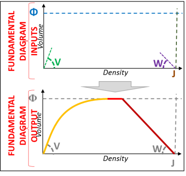
In this example, the top view represents the input parameters V…W. The bottom view shows the shape of the resulting curve.

The shape of the curve that represents the hypocritical branch of the diagram (left side of the curve) is parabolic. The shape of the hypercritical branch (right side of the curve), however, is linear.

Potentially, each link of the model can have a different fundamental diagram due to the variations of the 4 parameters. Two links have the same fundamental diagram only when they have the same parameters V, Φ, J, and W.

The following example illustrates how to define the attributes CapPrT and OutCapPrT.

Scenario 1: 4 lanes > 3 lanes

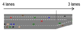
• CapPrT = 4 lanes × 2000 veh/(h lanes) = 8000 veh/h
• OutCapPrT = 3 lanes × 2000 veh/(h lanes) = 6000 veh/h
• UseOutCapPrT = true

Scenario 2: 2 lanes > 3 lanes

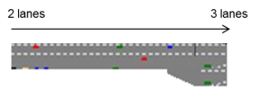
• CapPrT = 2 lanes × 2000 veh/(h lanes) = 4000 veh/h
• OutCapPrT = 3 lanes × 2000 veh/(h lanes) = 6000 veh/h
• UseOutCapPrT = true

If you consider a junction geometry, the output capacity of a single lane is determined in two different ways depending on the value of UseOutCapPrt.

UseOutCapPrt = true.

The lane capacity is equal to the OutCapPrT of the link divided by the number of head lanes (the number of lanes defined in the junction geometry):

OutCap Lane = OutCap Link/numHeadLanes

UseOutCapPrt = false.

The lane out capacity is equal to the link out capacity CapPrt divided by the link attribute NLAN:

OutCap Lane = CapPrt Link/NLAN

You can take into account traffic signals in the model just by using link parameters, without explicitly modeling the junction. Thus, you can skip defining main nodes and defining time-varying attributes on links, turns, and main turns.

In particular, you can use the following link UDAs created with PrepareVisumForOptima.net:

• GREN: effective green share of the signal at the To node
• CYCL: cycle time of the signal at the To node

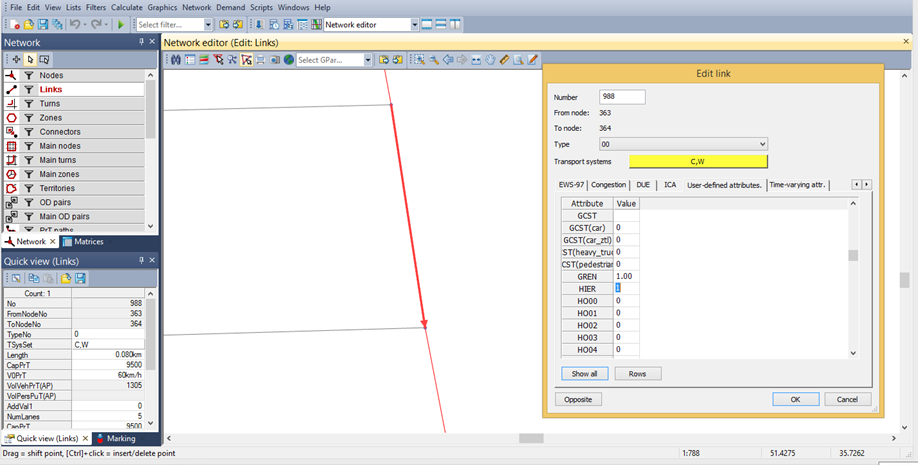
Procedure

To edit the parameters GREN and CYCL on links:

1. Activate the link layer.
2. Activate Edit mode.
3. Double-click the link to edit it.
4. Click the User-defined attributes tab.

5. Edit the attributes in the list.

   

Pros and cons

Modeling the effect of traffic signals on links is the simplest approach to represent traffic signals within the Optima model. It has the advantage that it requires only few input parameters.

On the other hand, a model created in this way might be too simple to properly describe cases:

• When the approach has many maneuvers controlled by different signal groups
• When the traffic plan of the signal changes significantly during the simulation
• When the traffic signals are synchronized on a road

Note that:

• If CYCL > 0 and GREN < 1, the link will experience a reduction of exit capacity (given by the GREN share) and an extra delay time that can be computed with the Webster Delay formula.
• If CYCL = 0 and GREN < 1, the link will also experience a reduction of the exit capacity.
• If GREN = 0, the link is closed.

Example

The following example shows 2 links with the same OUTCAPACITY and different signal values on the To node, estimating the corresponding Webster Delay.

Scenario 1:

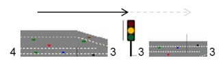
• CapPrT = 4 lanes × 2000 veh/(h lanes) = 8000 veh/h
• OutCapPrT = 3 lanes × 2000 veh/(h lanes) = 6000 veh/h
• GREN = 0.6 (60% green light)
• CYCL = 80 s
• SignalOutCap = OutCapPrT × GREN = 6000 × 0.6 = 3600 veh/h
• WebsterDelay (minimum, if f = 0) = 0.5 × CYCL × ( 1 − GREN)² = 6.4 s

Scenario 2:

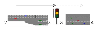
• CapPrT = 2 lanes × 2000 veh/(h lanes) = 4000 veh/h
• OutCapPrT = 3 lanes × 2000 veh/(h lanes) = 6000 veh/h
• GREN = 0.8 (80% green light)
• CYCL = 100 s
• SignalOutCap = OutCapPrT × GREN = 6000 × 0.8 = 4800 veh/h
• WebsterDelay (minimum, if f = 0) = 0.5 × CYCL × ( 1 − GREN)² = 2 s

Intersections with multiple approaches

In case of signalized intersections that have multiple approaches, you can replicate this methodology independently for each road approaching the signalized intersection.

In cases where it is important to model the different capacities of each maneuver at the signalized intersections, you can extend the approach of modeling the effect of traffic signals on links. This approach uses only link and turn parameters. In this case, you can skip modeling the junction geometry and you can skip modeling signal controls.

Sample scenario

Look at the following example to illustrate the methodology for estimating link and turn parameters used to model a road that approaches a signalized junction.

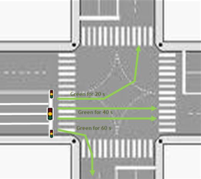
An eastbound road has 4 lanes along the link and 4 lanes at the intersection. At the intersection there are three independent signal lights:

• There is one signal light for the left maneuver with a green light for 20 seconds per cycle.
• There is one signal light for the straight maneuver with a green light for 40 seconds per cycle.
• There is one signal light for the right maneuver with a green light for 60 seconds per cycle.

The total cycle time of the intersection is 120 seconds.

There are different numbers of lanes:

• The left maneuver has 1 lane.
• The straight maneuver has 2 lanes.
• The right maneuver has 1 lane.

In the model, the link that represents the eastbound road should have the following parameters:

• CapPrT = 4 lanes × 2000 veh/(h lanes) = 8000 veh/h
• OutCapPrT = 4 lanes × 2000 veh/(h lanes) = 8000 veh/h
• GREN = average of the green share of the outgoing maneuvers, weighted by the number of lanes (alternatively by the measured flow on the maneuvers) = (( 20 s / 120 s ) × 1 lane + ( 40 s / 120 s ) × 2 lane + ( 60 s / 120 s ) × 1 lane )/ 4 lanes = 0.333
• CYCL = 120 s

It follows that:

• SignalOutCap = OutCapPrT × GREN = 8000 × 0.333 = 2664 veh/h
• WebsterDelay (minimum, if f = 0) = 0.5 × CYCL × ( 1 − GREN)² = 26.7 s

The outgoing turns should have the following parameters:

• CapPrT(left turn) = 1 lane × 2000 veh/h × ( 40 s / 120 s ) = 666.666 veh/h
• CapPrT(straight turn) = 2 lanes × 2000 veh/h × ( 50 s / 120 s ) = 1666.666 veh/h
• CapPrT(right turn) = 1 lane × 2000 veh/h × ( 60 s / 120 s ) = 1000 veh/h

This procedure must be replicated independently for each road that approaches the signalized intersection.