Smart Display methodology

The priority according to which the SD software sorts events, depends on several factors, such as:

Event severity and duration
The damage potentially produced by the event under normal traffic conditions
The number of road users who would be affected by the event
The distance between the variable message sign and the event

The response of SD consists of a set of messages of all relevant events, sorted by priority.

The set of messages can be reduced to a subset, based on threshold values.

Parameter	Description
ET	Set of the events
E	Set of the active events, E ⊂ ET
e	Generic event, e ∈ ET
S	Set of variable message signs
s	Generic variable message sign (real or virtual), s ∈ S
t	Current instant, t ∈ ℝ
ti_e	Starting instant of the event, e ∈ ET, ti_e ∈ ℝ
tf_e	Ending instant of the event, e ∈ ET, tf_e ∈ ℝ
A	Set of the links of the street graph
AE	Set of the links that contain at least one event, AE ⊂ A
a	Generic link of the graph, a ∈ A
A(e)	Set of the links on which there is the event e, e ∈ ET, A(e) ⊂ AE
a(e)	One of the links on which there is the event e, e ∈ ET, a(e) ∈ A(e)
a(s)	Link on which there is the variable message sign s, s ∈ S, a(s) ∈ A

By definition, active events are events for which their ending instant is either greater than the current instant or not specified.

Programmed events are events that have both their start time and their end time in the future. So they are also active events.

Thus, the system can provide information in advance with respect to the event start. Formally:

E = {e ∈ ET: tf_e ≥ t}

Message visualization priority

The visualization priority pv_se of a generic active event e on a generic variable message sign s is defined as:

pv_se = pi_e × pr_a(s)a(e)

where:

Parameter	Description
pi_e	Coefficient of the intrinsic priority of event e (disregarding a(s)). This relates to the severity of the event itself.
pr_a(s)a(e)	Coefficient of the relative priority with respect to variable message sign s. This relates to the probability of a vehicle located on link a(s) to encounter event e on its route.

Intrinsic priority of an event

The intrinsic priority pi_e of a generic event e is defined as a linear combination of the following parameters:

Parameter	Description
ie_e	Event importance
de_e	Event damage
pe_e	Event temporal distance

Event importance

The event importance ie_e is exogenously defined with an absolute value ie_e ∈ ℝ (→ Smart Display configuration > Event attributes).

Event damage

The event damage de_e is defined as the delay caused by a reduction of capacity rc_e or speed rv_e due to the event, namely:

where:

Parameter	Description
T₁	Maximum delay in seconds
rv_e	Share speed reduction in the interval [0,1] 0 = no reduction 1 = null speed
rc_e	Share capacity reduction in the interval [0,1] 0 = no reduction 1 = null capacity
L_a	Length of the link a
V_a	Maximum speed of the link a (Where not provided, def_sped is used)
C_a	Capacity of the link a
f_a	Estimated flow on the link a if available from offline simulations Else C_a / 2 is used

For details on the database attribute names, see: → Smart Display configuration.

Given an event e that sets absolute values of speed and / or capacity, the share reductions rv_e and rc_e from the original link values are computed as the worse among all the links to which the event e applies.

Given T₁ as an upper limit, the delay is computed from the available information with the formula shown above.

The first part of the formula comes from the delay due to a speed reduction, namely:

The second part of the formula is the average loss time in a bottleneck queue due to the capacity reduction, as described in the following example of the bottleneck queue.

Bottleneck queue example:

The event is active between the instants t_i and t_f. A queue forms while the event has an effect. The queue dissipates between the instants t_f and t. The next image depicts this scenario. On the x-axis, there is the time t. On the y-axis, there is the number of vehicles F = F(t):

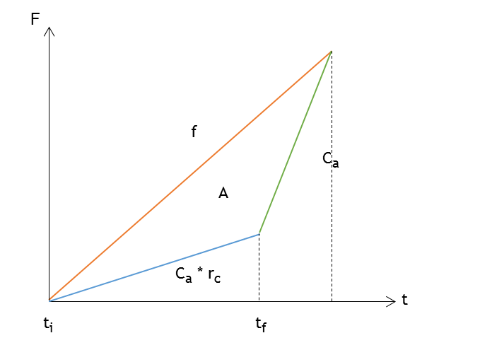
Now consider a constant flow of cars traveling between instants t_i ∈ t, represented by the orange straight line. Suppose there is an event within the interval [t_i, t_f] that reduces the street capacity. Then, in this time interval, the street capacity takes the value C_a × r_c, where r_c is a capacity reduction, 0 ≤ r_c ≤ 1). Next, the street capacity reverts to its original value during the time interval [t_f, t]. In the image, these two scenarios are described by the blue line and by the green lines.

The average delay is computed as the ratio between the area of triangle A and the number of vehicles that suffer the delay Nr = (t − t_i) × f.

Event temporal distance

The temporal distance pe_e is defined as the time between the current instant and the start time of the event, namely:

where TR is the maximum temporal distance of the event.

For the attribute names of the DB, see : → Smart Display configuration.

Calculation of the intrinsic priority

Finally, the intrinsic priority is calculated as:

pi_e = β_ie × ie_e + β_de × de_e + β_pe × pe_e

The coefficients β are configurable parameters. For the filed names of the database: → Smart Display configuration > Parameters.

Relative priority of an event

The relative priority between two generic links a and b, pr_ab, is defined as the traffic portion that, traveling from a, arrives at b. Therefore, the relative priority of an event e from link a, Prm(a,e), is computed by summing up pr_ab for each link b ∈ A(e) with the constraint that each link b has to belong to a different path so that each vehicle reaching any b from a is counted only once.

Additional definitions

Expression	Definition
tm(h, k)	Minimum travel time from the head (ending node) of the generic link h to the head of generic link k tm(h, k) ∈ ℝ+ h ∈ A k ∈ A
Ltm(a)	List of links in increasing order in respect to tm(a, h)
FST_a	Forward star of a, that is the set of links for which it is possible to turn into, coming from link a (the set does not contain any links for which there is a denied turn from a). This set is given and it represents the street network topology.
TotFlow(a)	Total flow on link a (estimated from the static assignment of the demand matrices of the standard day type)
currFlow(a,d)	Flow on link a, directed to destination d
currTurnFlow(h,k,d)	Flow on the turn from h to k, directed to destination d
tp_a	Travel time of the link a, computed as L_a / V_a
Sr_hk^d	Splitting rate (turning probability) from link h to link k with a fixed destination d (→ Splitting rate computation)
E(a)	Set of events that are on link a
Prm(a,e)	Relative priority of the message e in respect to link a
β_vms	Reduction coefficient of relative priority for traveling on a link on which there is a variable message sign β_vms ∈ (0,1)
α_tr	Reduction coefficient of the relative priority for the travel time α_TR ∈ (0,1)
T_TH	Time lag beyond which the events are not relevant and their priority is set to 0
P_TH	Threshold of flow percentage for the destination below which the search of events is stopped
AS	Set of links that contain at least one variable message sign
D	Set of the model destination zones

The efficient turn for a link a is defined as:
SE(a) = {(h,k) ∈ AxA: tm(a,h) < tm(a,k)}

Algorithm

#======================================================================
# Initialization
#======================================================================

# a <-- Link on which the request is done (external INPUT)

# If an event is not on a link (street of the primary network), it is 
# associated to the closest zone (Euclidean distance)
FOR e ∈ E
    IF e IS NOT on graph model
        ProjectEventOnNearestDestinationZone(e)
    ENDIF 
NEXT

# If the link a does not belong to the model or if it is on a link of 
# the model on which there is no flow, then find the closest link of 
# the model on which there is a positive flow
a = FindNearestLinkWithFlow(a)

# Travel time initialization and probabilities initialization on all 
# the links except the one in input, for each destination
tm(a,k) = ∞, Ɐ k ≠ a
pr(k,d) = 0, Ɐ k ∈ A, d ∈ D

# Travel time initialization on the input link
tm(a,a) = 0

# Set the priority of all events to zero
prm(a,e)=0  Ɐe ∈ ET

#=====================================================================
# Propagation
#=====================================================================

# Cycle over all destinations
For d ∈ D

# Initialization of the list with the input link
    Ltm(a) = {a}

# Initialization of the probability to reach the destination d 
# starting from the link a
    pr(a,d) = currFlow(a,d) / TotFlow(a)

# While the list is not empty or while not all events have yet been 
# reached 
    DO UNTIL Ltm(a) = Ø 
        Pop the first link in the list
        h: tm(a,h) = min{ tm(a, k), k ∈ Ltm(a)}
        Ltm(a) = Ltm(a) \ {h}

        For each link k belonging to the forward star of h
        FOR k ∈ FSTh

# Compute the probability, for going from link a to destination d
# over link h and link k,
# as the probability of having reached h from a, times the 
# probability to turn from h to k, in case of heading to 
# destination d
            prob_k = pr(h,d) * Srhkd

# If the probability is not zero and greater than the propagation 
# threshold configurable from the commandline
            IF prob_k > 0 AND prob_k > PTH
                if on link k there is a variable message sign
                IF k ∈ AS 
                   prob_k = prob_k ∙ β_vms
                ENDIF

# Update the probability to reach link k, starting from 
# destination d 
                pr(k,d) += prob_k

# For each event on link k, update the probability to reach
# the event, if this has not yet been reached, summing prob_k 
                FOR e ∊E(k)
                    prm(a,e) += prob_k
                NEXT

# If link k is not in the list or if the probability
# to reach this link is not zero and greater than the configurable
# threshold and if, moreover, the time of reaching its head
# is minor than the time configurable threshold, then update the 
# reaching time of k or insert the link into the list
                IF ( k is not element of Ltm(a) OR 
                     (pr(k,d) > 0 AND 
                      pr(k,d) >= PTH AND                  
                      (tm(a,h) + tm(h,k)) < TTH) )

                    tm(a,k) = tm(a,h) + tpk
                   IF ( k is not element of Ltm(a)
                       Ltm(a) = Ltm(a) ᴗ {k}
                    ENDIF
                END IF
            END IF
        NEXT k
    LOOP
Next d

# Compute the maximum and minimum reaching time of the events 
# required to rescale the relative probabilities of the events
T_MAX = 0
T_min(e) = Inf Ɐ e ∈ E
FOR e ∈ E
    FOR k ∈ A(e)
        IF tm(a,k) > T_MAX
            T_MAX = tm(a,k)
        END IF

        IF tm(a,k) < T_min(e)
            T_min(e) = tm(a,k)
        END IF
    NEXT
NEXT

FOR e ∈ E
    IF TTH > 0 AND T_min(e) > TTH THEN 
        prm(a,e) = 0
    ENDIF

    prm(a,e) *= (1 +α_tr∙(T_MAX-T_min(e))/T_MAX)
NEXT

The algorithm terminates when one of the following conditions is met:

All events have been reached
All links of the graph reachable from a(s) have been visited
The time threshold T_TH for the probability propagation is exceeded
The probability has decreased below the threshold P_TH on the whole exploration border of the graph

Note that, given a variable message sign s, the algorithm computes the relative priorities towards all the active events.