Map matching algorithm
The map-matching algorithm works incrementally. When a new point of a given trajectory is available, the algorithm retrieves all previous data of the trajectory and rebuilds the map-matched path considering the new point.
The new path can be very different from the old one because it does not simply expand the old path. A score value can be associated to each map-matched trajectory. Each time a new point is taken into account, the algorithm generates N new paths sorted according to the score value. The lower the score value is, the better is the map-matched trajectory.
At each iteration, a new sorted set of best paths is created, expanding all paths stored in the previous sorted set. The expansion of a path consists in exploring the forward star of the last street arc and subsequent arcs. (The stopping criteria of this expansion will be described later.) Each new visited street arc produces a new path that is inserted into the new trajectory sorted set. When all old paths have been expanded, the new sorted set (with only the first N best paths) replaces the old one, and the trajectory is ready to be improved by a new incoming GPS point.
When a trajectory is built for the first time (so when the first GPS point is coming in) the sorted set of trajectory data is filled with all street arcs that are part of the forward star and backward star of all nodes that belong to a circle area centered around the GPS point itself. The score of these starting trajectories is given only by the distance between the GPS point and the corresponding street, so only the contribution is considered (see the following section for details on contributions).
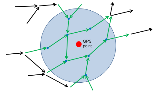
Given a GPS point (red dot) from which a new trajectory has to be created, a circle around this GPS point (blue area) is considered. For all nodes of the graph inside this area (blue dots), every incoming and outgoing street arc (green arrows) is considered for creating the first set of trajectories.
The score of a trajectory T is defined as a weighted sum of 5 contributions
where p is the p-th point out of K defining the trajectory, and wi is the weight of the contributions.
The individual contributions that define the global score of a trajectory are:
| Score Contribution | Brief description (for details see subsections below) |
|---|---|
| Distance between the GPS point and the matched arc | |
| Difference between the time needed to cover the path connecting two consecutive GPS points and the time span of the input timestamps of the same points | |
| Difference between the linear distance (as the crow flies) between two consecutive GPS points and the length of the path covered on the graph between the projection feet of these two points | |
| U-turn penalty | |
| Angle between the direction defined by two consecutive GPS points and the direction identified by the last piece of the map-matched trajectory |
The weight of each contribution can be configured.
score
The score is meant to match the nearest street to the given GPS point.
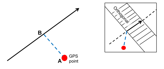
Given a GPS point that is associated with a street, the orthogonal projection segment AB (dashed blue line) is the score .
Note that if the GPS point is outside the orthogonal band defined by the street itself, the projection segment connects the From node or the To node of the street (see image detail).
score
The score is meant to match streets for which the travel time along the map-matched path (computed using the base speeds) is most similar to the elapsed time measured from the GPS timestamps.
Note that this score prefers uncongested streets over congested ones.
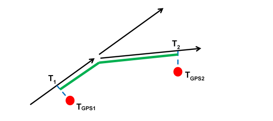
Given two consecutive GPS points, the score is computed as the difference between the elapsed time of the two GPS timestamps, and the time needed to cover the matched path (green line) between the feet of the projected GPS points.
score
The score is meant to minimize the total travel distance, making it as similar to the linear distance (as the crow flies) as possible.
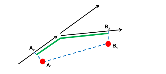
Given two consecutive GPS points, the score is computed as the difference between the linear distance of the two GPS points (dashed blue segment) and the matched path length (green line) between the feet of the projected GPS points.
where L(P,Q) is the distance of the polyline connecting points A2 and B2.
score
The score is meant to penalize U-turns.

Given the three points T1, T2, and T3, the blue path has to be compared to the green one in order to select the best map match. The green path contains the U-turn penalty that is proportional to the travel time needed to go from the To node of the arc a to the point T2 (dashed red double arrow).
score
The score is meant to prioritize paths for which the travel direction is as similar as possible to the path defined by the line connecting the GPS points.
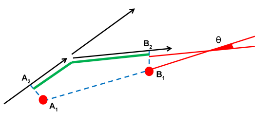
Given two consecutive GPS points, the score is proportional to the angle θ between the line connecting the two GPS points and the line identified by the last piece of the map-matched trajectory.
The trajectory score is the sum of different terms. In order to obtain an overall meaningful score it is important that all terms are of the same order of magnitude. For this reason, the software uses some constant factors to homogenize the sum. In addition, various configuration parameters let you tune almost all terms of the score function.
The most appropriate way of setting the configuration values for these parameters is to:
- Map match several trajectories
- Tune the parameters
- Select those parameters for which all matches (or at least a great proportion of the matches) are satisfactory from a human point of view
Essentially, this is an iterative, supervised approach for calibrating the parameters.
The map-matching algorithm works incrementally, so each time a new GPS point arrives (except for the first one), old matched paths are expanded in order to build a new set of paths.
Expansion strategies
For each path of the old set, a new path is created by associating the new GPS point with the last segment of the old path. After that, the expansion can proceed using one of the two following strategies, depending on the configuration of the software:
- Expansion strategy 1: If the last GPS point is associated near the end of the last street of the previous path, for each arc of the forward star of this last street a new path is created.
- Expansion strategy 2: Regardless of the first association, for each arc of the forward star of the last street of the previous path a new path is generated if the foot projection of the last GPS point on the arc is less than 1. A new expansion starting from this new arc is performed in a recursive manner if the foot projection is greater than 0.
Foot projection
The foot projection is the signed ratio between the length of the projected vector that connects the From node of the street with the GPS point along the street and the length of the street itself. The sign is positive if the projected vector has the same direction as the street.
The following figure illustrates the GPS foot projection: S is the length of the street. L is the length of the projection of the vector (blue arrow) connecting the From node of the street and the GPS point. θ is the angle between the street and the vector.
Alpha indicates whether the GPS point's position is before or after the directed street S.
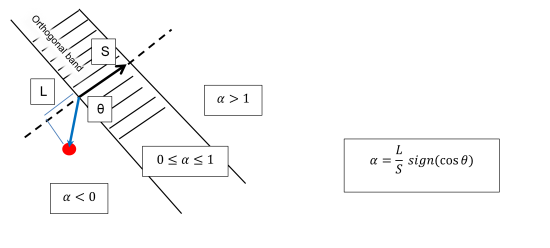
For a better understanding, the next two figures show some examples of how is computed. Street arcs with a green halo have , while those with a red halo have . For the other arcs, and the projection line is shown (blue line).

Non-recursive path expansion vs. recursive path expansion
Expansion strategy 1 is non-recursive. It always produces a finite small number of new paths.
Expansion strategy 2 is recursive and could thus produce many new paths. So the stopping criteria are very important here.
The next images show an example of the non-recursive path expansion vs. two examples of the recursive method. For the recursive examples, the stopping criteria must allow to approach the new GPS point and they must stop the process when we are moving too far away from the new GPS point. Also the algorithm must avoid infinite looping over the same streets.
The stopping criteria are built based on the value of . When is less than or equal to 0, the corresponding link is no longer expanded.
Non-recursive path expansion
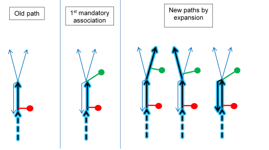
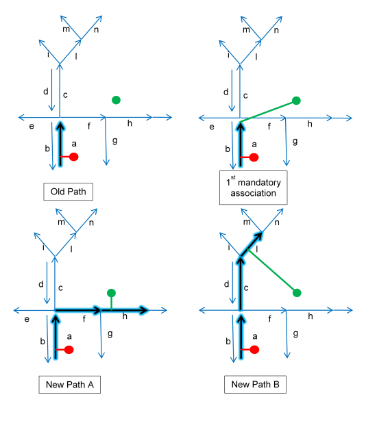
On the left section of the next image, you see the starting path (blue halo) that is going to be expanded.
In the middle section of the image, the new GPS point (green dot) is associated with the last link of the old path. This new path is added to the set of new paths.
In the right section of the image, the forward star of the last link of the old path is explored and the new GPS point is associated to each outgoing link, creating a new path for each link.
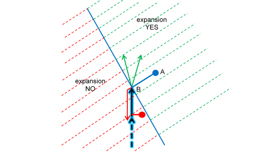
Given a path (blue halo) and a new GPS point (blue dot), expansion is allowed only for those links (green arrows) of the forward star of the last arc of the path that are pointing towards the green half-plane region . This region is defined by the orthogonal line to the segment that joins the new GPS point (A) with the To node of the last arc (B). These criteria allow an expansion in the direction of the new GPS point until it is not overcome.
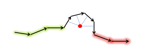
Based on the recursive expansion, the new GPS point (green dot in the next image below) produces three new paths A, B, and C, highlighted with a blue halo. After the first mandatory association, the forward star of the link a is composed by the links b, c, e, and f. However, only the links c and f can be expanded. So, taking f, only the link h can be expanded again. Then the recursion stops, producing the path A (a→f→h). While taking c, its forward star can be expanded into l and d. So, following l the recursion stops immediately, creating the new path B (a→c→l). Following d, its forward star can be expanded only into f, and the recursion produces the new path C (a→c→d→f→h).
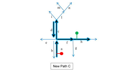
While creating path C, the algorithm makes an important check to avoid infinite recursion. Actually when the link d needs to be expanded, the allowed forward star is composed of the links f and c. While taking f is fine, using c produces an infinite loop over the links c and d (a→c→d→c→d→c→d→…). This issue is avoided by imposing that the path that we are building does not contain any duplicated links.
Important considerations
-
Loops:
Note that recursive path expansion does not avoid creating paths with loops. However, the imposed constraint that stops infinite recursion can produce no more than one loop between two consecutive GPS points (as shown in the previous image). In principle, it is OK if the map-matching creates looping paths. Usually looping paths are discarded because they have higher scores than straight paths.
-
Sampling rate:
The Marchal algorithm is well suited for high-frequency-rate GPS points.
The non-recursive expansion procedure will fail for low sampling rates, mainly because the expansion has a depth of only one step. For this reason, the recursive expansion method needs to be preferred in these situations. However, if two consecutive points are very far away from each other, the recursive expansion method has the drawback that the computational effort can be very high because a lot of new paths can be produced. In this case, a shortest path approach must be used.
Vehicle Tracker has a configuration setting for which an A* shortest path search is performed when the linear distance between two consecutive points exceeds a given threshold. The algorithm has been designed to seamlessly switch between the expansion approach, whatever it is, and the shortest path approach.
-
Performance optimization
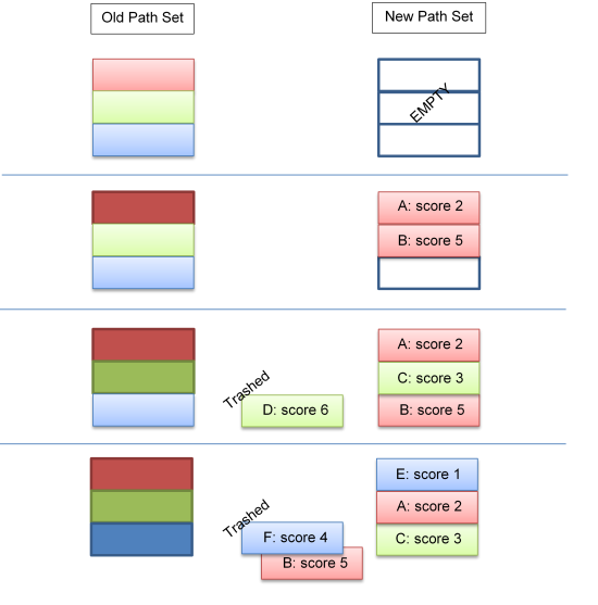
As said before, the algorithm works incrementally: It takes the old set of best paths, expands them all, and takes the new best N in terms of score to create the new set.
For memory and performance reasons, this operation is not performed exactly as described (that is first creating all new paths, then sorting by score and keeping the best N). The new set of paths has the fixed capacity of N. Each time a new path is generated, it is inserted into the new set. The insertion uses an insertion sort algorithm if either the set is not yet full or if the score is better than the worst score actually within the set.
The next image illustrates the strategy for creating the new set of paths from the previous set. Each colored box represents a path. Dark colors indicate that the path is expanded and the newly generated paths are inserted into the new set.
The recursive expansion algorithm becomes less accurate in situations where the GPS points are going towards a direction opposite to the path on the graph.
Example: The trajectory goes on the left but due to the topology of the graph you are forced to use streets that for a while go on the right. The following figure illustrates a scenario that involves a roundabout, and the figure below shows a scenario that involves a highway ramp. In both cases, the expansion stops prematurely and an accumulation of GPS points on top of the old path is created. This produces a low speed value on the end of the old path (which is clearly an error). Also note that if the expansion is recovered, it may happen that the distance covered from the last accumulated GPS point and the first unblocked point is very large so that the speeds computed on the streets between these two points can be very high (which is clearly an error, too).
Example: Roundabout
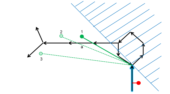
The actual trajectory is highlighted with a blue halo. When the new GPS point arrives (filled green dot) it is matched on the To node of the path but it is not able to expand itself, creating a new path going via the roundabout to the link a. Moreover, if new GPS points arrive (dashed light green dots) and if these GPS points are outside the blue region (as defined by the stopping criteria, see figure in subsection on recursive path expansion), they will all be matched on the To node of the old path without expanding anything. The expansion will be recovered if a new point is within the blue region and if the path was not cut due to too big a linear distance (configurable) between the To node of the old path and the actual GPS coordinates.
Example: Highway ramp
The actual trajectory is highlighted with a blue halo. When the new GPS point arrives (filled green dot) it is matched on the To node of the path. However, it is not able to expand itself, creating a new path proceeding on the ramp until the link a. The behavior is the same as for the roundabout described above.