The following describes the general scheme of the fixed point problem that formalizes the Dynamic Traffic Assignment (DTA) problem, as modeled in TRE.
The key feature of the scheme is the different time discretization:
- It is less detailed on the demand side of the equilibrium problem, namely the route choice;
- It is more detailed on the supply side, namely the dynamic network loading.
This separation allows for a balanced investment of computing resources on the two sides of the equilibrium problem.
For a detailed description of the supply implementation: → Traffic model.
Route choice in the supply implementation is based on given local undirected splitting rates. This means that the turn probabilities at each node are evaluated without explicitly taking into account the destinations of vehicles. The splitting rates then become the pivot variables between the two models and represent the fixed-point-problem variables.
For given OD flows, DTA consists of seeking a path flow pattern consistent with the costs returned by the network performance model. DTA can be formalized as a fixed-point problem in terms of splitting rates.
DTA has its own gap function (see → TRE convergence formulas), measuring the error on the DTA problem.
Scheme
The next image describes the logical scheme of the DTA problem:
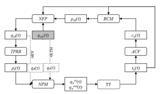
The scheme consists of the following functional components and variables:
| Component | Description |
|---|---|
| ACF | Arc Cost Function. Gets user perceived costs. |
| RCM | Route Choice Model. Computes od shortest paths. |
| NFP | Network Flow Propagation. Computes expected arc flows. |
| TPRB | Aggregation and ratio. Gets non-destination-based turn probabilities. |
| NPM | Network Performance Model. Computes congested arc flows. |
| TT | Travel Times. Computes travel times. |
| Variable | Description |
|---|---|
| ca(τ) | Cost of arc a for users entering it at time τ |
| ptd(τ) | Turn probability of turn t at time τ for users traveling toward d |
| qod(τ) | Flow of users departing at time τ traveling from origin o to destination d |
| qtd(τ) | Flow of turn t at time τ of users traveling toward d, resulting from the NFP |
| pt(τ) | Turn probability of turn t at time τ |
| qo(τ) | Flow of users departing from origin o at time τ |
| qa(τ) | Flow of users entering link a at time τ, resulting from the NFP |
| qain(τ) | Inflow of arc a at time τ, resulting from the NPM |
| qaout(τ) | Outflow of arc a at time τ, resulting from the NPM |
| ta(τ) | Travel time of arc a for users entering the arc at time τ |
Two kinds of arc flows are considered in the model:
-
The arc flow produced by the network flow propagation model on the basis of route choices to determine the splitting rates. This arc flow is consistent with drivers’ behavior but inconsistent with congestion phenomena.
- The arc flow produced by the dynamic network loading model for given splitting rates. This arc flow is consistent with congestion phenomena but inconsistent with drivers’ behavior.
Only at equilibrium, these two variables become mutually consistent, although they are referred to two different discretizations used for time aggregation: the DTA interval (of some minutes) and the simulation intervals (of a few seconds).
The supply model at each iteration computes the network performance from given splitting rates (→ Traffic model). The travel times are then updated and route choices can subsequently be recomputed. In the DTA problem, this loop occurs until a stop criterion is met.
The DNL (Dynamic Network Loading) problem is a simplified version of the DTA problem, in which route choices are never recomputed. With reference to the scheme above, the DNL problem skips steps of ACF and RCM, and just updates the expected flows via NFP, consistently with the new updated travel times from the TT. From the point of view of the definition of DTA, the DNL can be defined as follows:
For given OD flows, DNL consists of seeking a path flow pattern consistent with the travel times returned by the network performance model. DNL can be formalized as a fixed-point problem in terms of splitting rates.
It is suggested to run some iterations of DNL at the end of the DTA iterations, to give the resulting simulation a higher consistency between the expected flows – output of the NFP – and the congested ones – output of the NPM –. Note that with respect to the DTA, the DNL has its own gap function (see → TRE convergence formulas), measuring the error on the DNL problem. This can be used to assess the convergence of the final DNL iterations.
The convergence algorithm determines the capability of the algorithm to reach an equilibrium fixed-point. Two alternative methods can be used:
-
MSA (Method of Successive Averages): the MSA is an easy-to-apply convergence algorithm, proved to reach equilibrium in a great-enough number of iterations. It is one of the most common convergence algorithms in traffic assignment problems. During intermediate iterations it contains also non-sense route choices that occurred in previous iterations.
Important: Currently MSA is deprecated, but it is maintained in Optima for backward compatibility.
- GP (Gradient Projection): the GP is an advanced optimization algorithm, recently introduced in many application fields. It is an evolution of the convergence algorithm used in LUCE. GP is based on Temporal Layer Algorithm (see the parameter AssignmentAlgorithm → Equilibrium parameters).
Both are non-monotone descent algorithms, so worse intermediate steps are admitted.